11 minutes
FITE7410 Financial Fraud Analytics Techniques (Part 1)
.png)
Financial Fraud Analytics
Fraud detection models
- classification
- the output is category
- regression
- the output is a real value
Techniques
- statistics techniques
- break-point analysis
- peer-group analysis
- association rule analysis
- linear/logistic regressions
- AI/DM/ML techniques
- supervised learning
- using historical information to retrieve patterns
- required labelled dataset
- unsupervised learning
- using historical information to retrieve patterns
- do not require labelled dataset
- divided into
- clustering - to discover the inherent groupings in the data
- association - to discover rules that describe large portions of the data, find relation
- semi-supervised learning
- deal with pertially labelled data
- social network analysis
- learn and detect characteristics of fraudulent behavior in a network of linked entities
- notes
- these techniques are not mutually exclusive but complement each other
- an effective fraud detection and prevention system may combine the use of different techniques
- supervised learning
Data analytics
- predictive analytics
- logistic regression
- decision tree
- random forest
- neural network
- support vector machines
- descriptive analytics
- clustering
- autoencoder
Statistics Techniques
Descriptive analytics for fraud detection
- outlier detection techniques
- break-point analysis
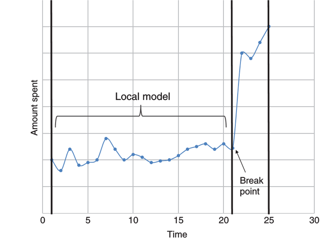
- intra-account, indicates by a sudden change in account behavior
- starts from defining a fixed time window
- split the time window into old and new
- old part represents the local model or profile against which the new observations will be compared
- use t-test (mean comparison) to compare the averages of the old and new parts
- observations are ranked according to the t-statistical value
- peer-group analysis
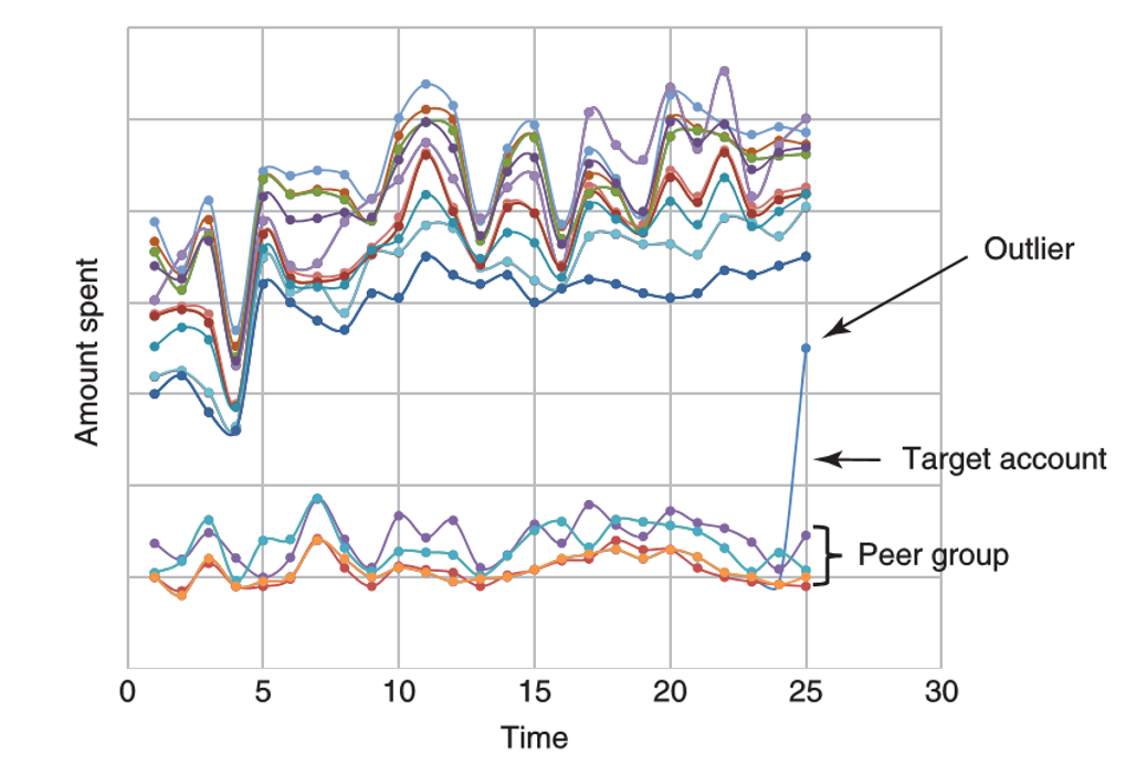
- inter-account, compare with peer-group (nomal behavior)
- identifies the peer group of a target account
- by using prior business knowledge or in a statistical way
- group size cannot be too small (sensitive to noise), or too big (insensitive to local irregularities)
- compares the behaviors of target account with peer accounts, e.g. t-test, any distance metrics
- disadvantage
- the two methods can be used to detect local anomalies rather than global anomalies
- cases may be normal in global population
- these cases are marked as suspicious when compared to local profile or peers (more sensitive to local anomalies)
- the two methods can be used to detect local anomalies rather than global anomalies
- break-point analysis
- relation detection techniques
- association rule analysis
- detect frequently occurring relationships between items
- originates from market basket analysis - to detect which items are frequently purchased together
- rules measure correlation associations, should not be interpreted as casual relation
- steps
- identify frequent item sets
- frequency of an item set is measured by means of its support \(support(X) = \frac{number \ of \ transactions \ supporting (X)}{total \ number \ of \ transactions}\)
- example
- item set {insured A, police officer X, auto repair shop 1}
- occurs in claim ID# 1, 6, 9
- support = 3/10 = 30%
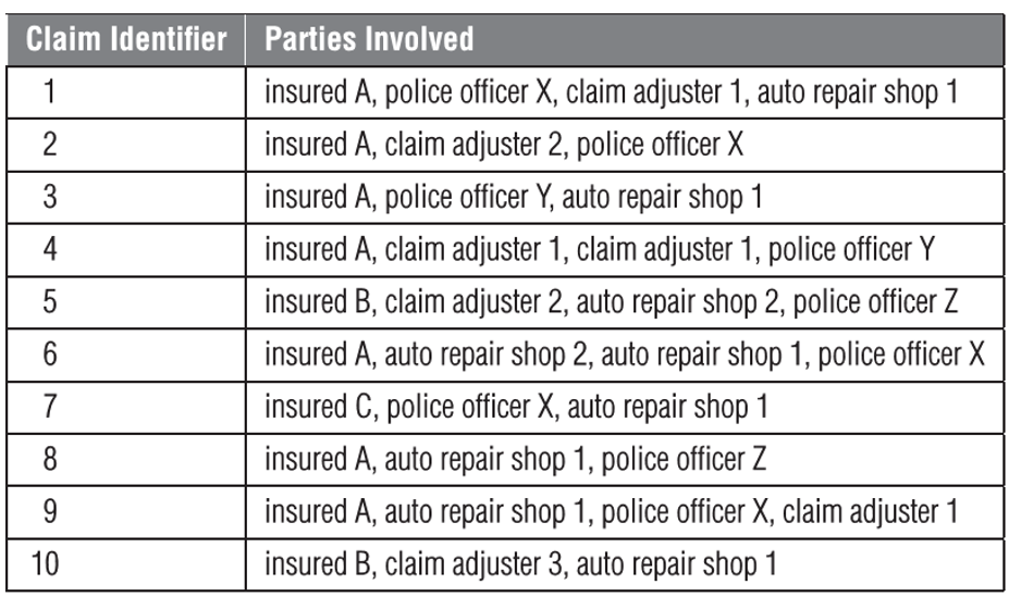
- a frequent item set - an item set of which the support is higher than a minimum value (e.g. 10%)
- identify association rules
- strength of the association rule measured by confidence \(confidence(X \rightarrow Y) = P(Y|X) = \frac{support(X \cap Y)}{support(X)}\)
- example
- item set {insured A, police officer X, auto repair shop 1} can have multiple association rules
- if insured A AND police officer X -> auto repair shop 1
- X = {insured A, police officer X}
- \(support(X) = 4/10\) (ID# 1, 2, 6, 9)
- Y = {auto repair shop 1}
- \(support(X\cap Y) = 3/10\) (ID# 1, 6, 9)
- confidence (X -> Y) = 75%
- if insured A AND auto repair shop 1 -> police office X
- if insured A -> auto repair shop 1 AND police office X
- if insured A AND police officer X -> auto repair shop 1
- item set {insured A, police officer X, auto repair shop 1} can have multiple association rules
- selected association rule - a rule of which the confidence is higher than a specified value
- identify frequent item sets
- association rule analysis
Predictive analytics for fraud detection
- linear regression
- used to model a continuous target variable
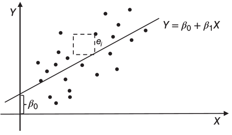
- general formulation:
\(Y = \beta_0 + \beta_1 X_1 + \cdots + \beta_N X_N\)
- slope: positive or negative relation between X and Y
- \(\beta_1\ldots\beta_N\): regression coefficient of a variable
- \(\beta_0\): intercept coefficient, excepted mean value of Y when all X = 0
- minimize the sum of all error squares (MSE = mean square error) to find the best fit straight line
- advantages
- performs exceptionally well for linearly separable data
- operationally efficient and easy to interpret & implement
- extrapolation beyond a specific dataset
- disadvantages
- target and exploratory variables must be of linear relation
- prone to noise and overfitting (a better fitting of the training dataset than the testing dataset)
- sensitive to outliers
- assumes exploratory variables are independent, might have problem of multicollinearity
- some variables are correlated, may have errors
- logistic regression
- can be used for classification problem where the target variable assumes a value between 0 or 1 (boundaries)
- \(P(Y=1)=1-P(Y=0)\)
- steps
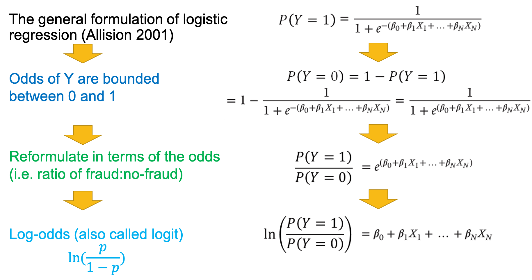
- optimize the maximum likelihood estimation (MLE) - chooses the parameters in such a way as to maximize the probability of getting the sample at hand, in order to find the best fit straight line
- interpret result
- linear in log odds (logit)
- estimates a linear decision boundary between the two classes
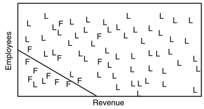
- advantages
- performs exceptionally well for linearly separable data
- operationally efficient and easy to implement
- a good baseline to measure performance of other more complex fraud detection model
- disadvantages
- nonlinear problem cannot be solved
- prone to overfitting
- difficult to capture complex relationships
Decision Tree
Overview
- basics

- aims
- minimize "impurity" in the data
- impurity
- the node impurity is a measure of the homogeneity of the labels at the node

- the node impurity is a measure of the homogeneity of the labels at the node
Splitting decision
categorical variables - decision tree
- Gini impurity
- entropy
example
- formula
\[IG(D_p,f)=I(D_p)-\frac{N_{left}}{N}I(D_{left})-\frac{N_{right}}{N}I(D_{right})\]
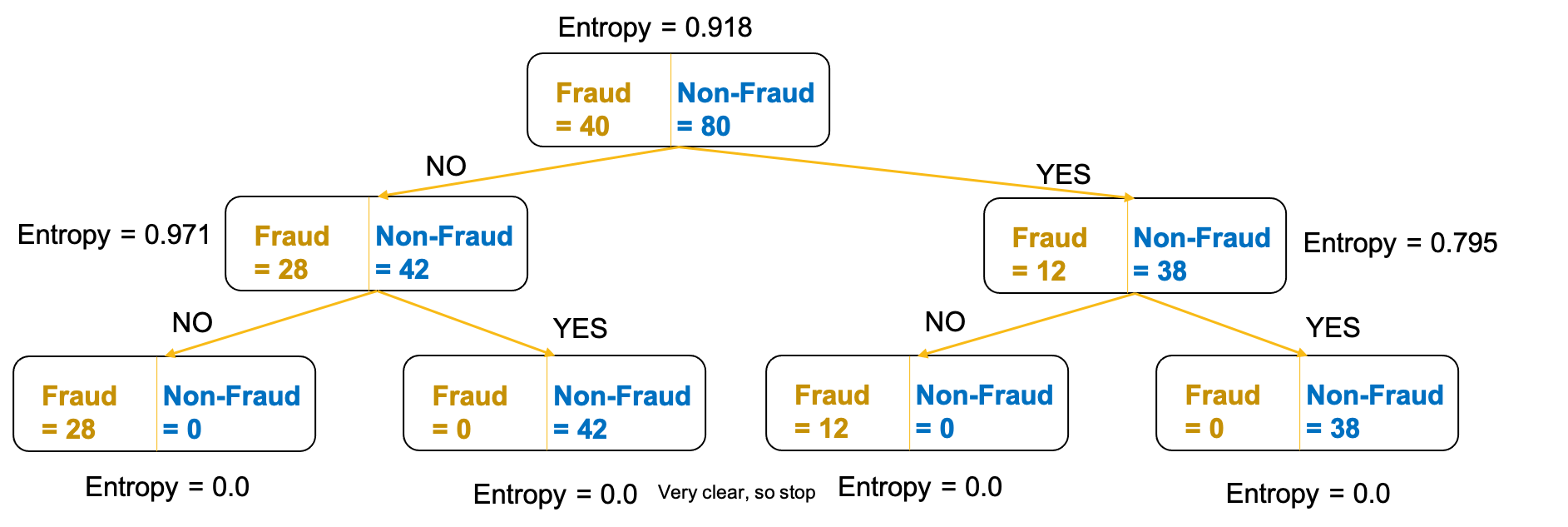
- compare the IG for splitting decision using the attribute "AGE" and "INCOME"
- IG(AGE) > IG(INCOME) -> use AGE as the splitting attribute

- formula
continuous variables - regression tree
- mean square error (MSE)
- variance
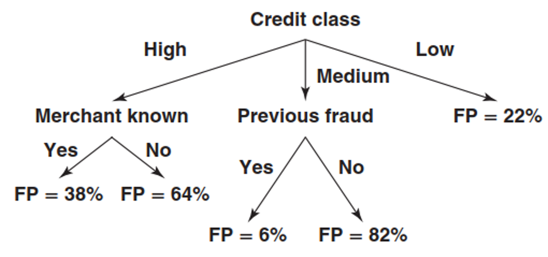
- regression tree splits - favour homogeneity within node and heterogeneity between nodes
- example - favour low MSE in a leave node
Stopping decision
- aims
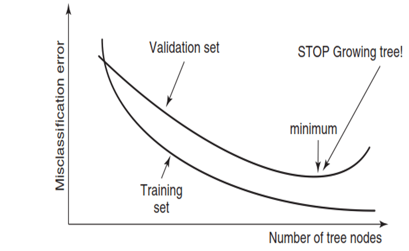
- avoid overfitting, the tree would be too complex and fails to correctly model the noise free pattern or trend in the data
- steps
- split the data into training set and validation set (usually 7:3)
- stop growing the tree when the misclassification error for validation set reaches its minimal value
Comparison
- advantages of decision tree
- easy to understand and interpret
- useful in data exploration
- less data clearing required - robust to outliers in inputs and no problem with missing values
- data type not a constraint - can handle both continuous and categorical data for both input and target data
- automatically detects interactions, accommodates nonlinearity and selects input variables
- disadvantages of decision tree
- prone to overfitting
- splitting turns continuous input variables into discrete variables
- unstable fitted tree - small change in the data result in a very different series of splits - sensitve to the dataset
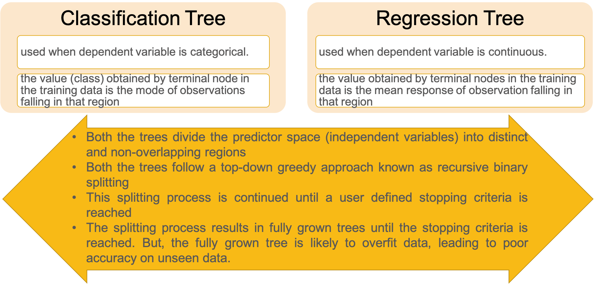
- classification vs regression tree
Ensemble Methods
Overview
- definition
- a machine learning model that involve a group of prediction models (not only one model)
- reasons of using ensemble learning
- performance: better predictions than any single contributing model
- robustness: reduce the spread or dispersion of the predictions and model performance
Bootstrap sampling
- definition
- smaller sample of same size are repeated drawn, with replacement, from the larger original sample
- procedures
- choose a number of bootstrap samples to perform
- choose a sample size
- for each bootstrap sample
- draw a sample with replacement with the chosen size
- calculate the statistic on the sample
- calculate the mean of the calculated sample statistics

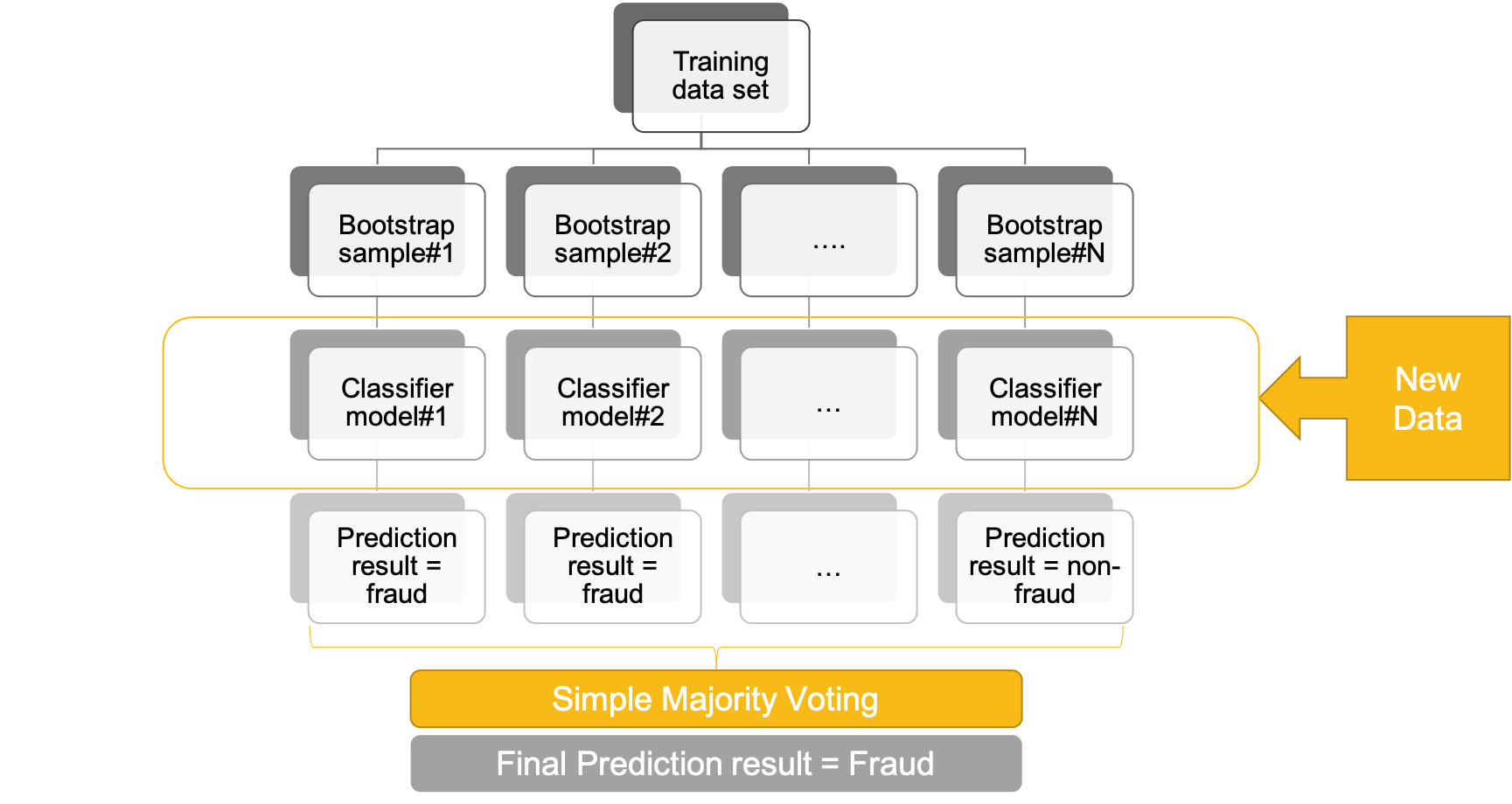
- bagging (bootstrap aggregating)
- take N number of bootstraps from the underlying sample
- build a classifier
- for classification -> major voting
- for regression -> calculate the average of the outcome of the N prediction models
Random Forest
Overview
- definition
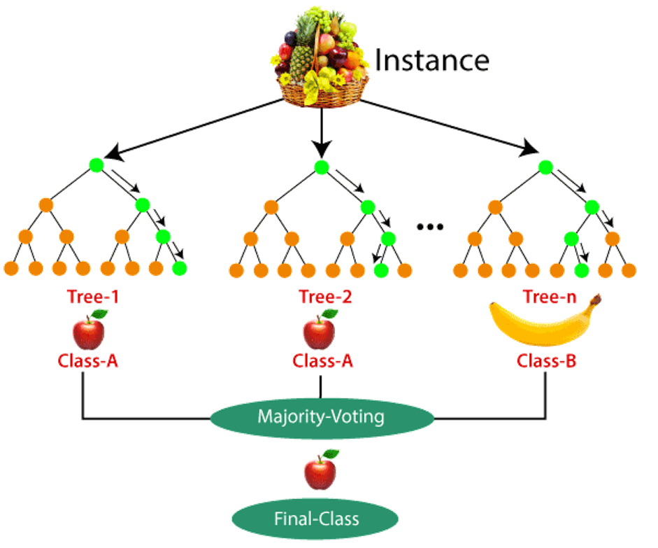
- is a forest of decision trees
- can be used for both classification tree and regression tree
- achieve dissimilarities among the decision trees by
- adopting a bootstrap procedure to select training samples for each tree (the same dataset -> useless)
- selecting a random subset of attributes at each node
- training different base models of decision trees
- result of random forest is a model with better performance compared to a single decision tree model
Comparison
- advantages
- random forest can achieve excellent predictive performance and suitable for the requirements of fraud detection
- capable of dealing with data sets having only a few observations, but with lots of variables
- disadvantages
- it is a black-box model, more complicated actually
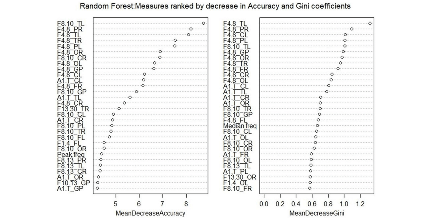
- variable importance can be used to understand the internal workings of random forest (or any ensemble model)
- it is a black-box model, more complicated actually
Variable importance
- aims
- when get result from random tree, which variables have the most predictive power
- variables with HIGH importance can be used for further analysis, while variables with LOW importance can be discarded
- example - provide two mechanism, which one should be used, it depends
Performance Evaluation
Split the sample data
- training dataset
- training data - to build the model
- validation data - to be used during model development (e.g. making stopping decision in decision tree)
- testing data - to test the performance of the model
- splitting the dataset
- observations used for training should not be used for testing or validation
- training:(validation):testing (not strict, it depends)
- 7:3 (validation dataset is not required)
- 4:3:3 (validation dataset is required)
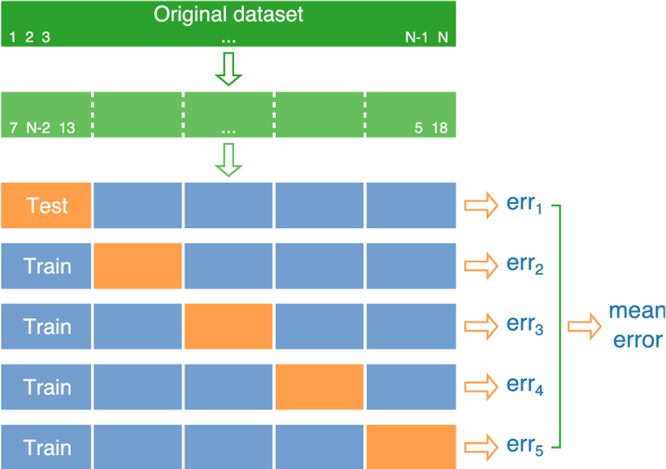
- k-fold cross-validation
- can be applied when the sample size is small
- procedures (k = 5)
- original dataset (shown in dark green) is randomly partitioned into k disjoint sets (shown in light green)
- then k − 1 parts are used for training a model (shown in blue) and remaining part is used for evaluation (shown in orange)
- this process is repeated k times for all possible choices of the test set, producing test errors
- the final performance is reported by averaging the errors from each iteration
- with more than one trained model, which one should be chosen
- similar to ensemble method, use voting procedure
- use leave one out cross-validation and randomly select one model
- randomly select
- using all data except dropped one for training
- since all models differ by one observation only, the performance should be similar for all models
- use all observations for training
- then, use the cross-validation performance result (mean error) as the independent estimate of the model
- only use when the sample size is really extremely small (no choice option)
Model evaluation
classification model
- statistics measure
- correlation tests
- comparison of mean tests
- regression tests
- non-parametric tests
performance metric
- mainly used in machine learning evaluation
the confusion matrix
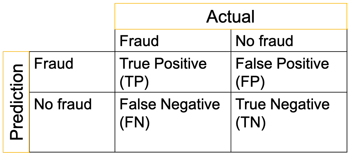
- accuracy: percentage of total items classified correctly
\[Classification\ accuracy=\frac{TP+TN}{TP+FP+FN+TN}\]
- error: percentage of total items classified incorrectly
\[Classification\ error=\frac{FP+FN}{TP+FP+FN+TN}\]
- recall: how many fraudsters are correctly classified as fraudsters (most important, i.e. favour TP > FN)
\[Sensitivity=Recall=Hit\ rate=\frac{TP}{TP+FN}\]
- precision: how many predicted fraudsters are actually fraudsters (useful if the objective is not to leave out important information, e.g. spam mail detection, i.e. TP > FP)
\[Precision=\frac{TP}{TP+FP}\]
- F1 score: the weight average of precision and recall (take into account FP and FN, thus more informative than accuracy)
\[F-measure=\frac{2\times (Precision\times Recall)}{Precision+Recall}\]
- for fraud detection models, recall is most useful performance measure
example
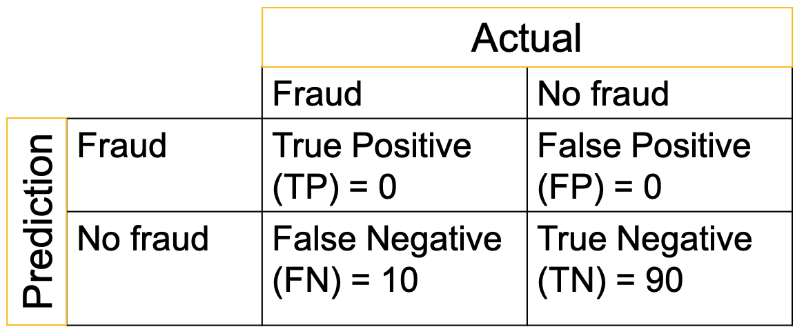
\[Accuracy = \frac{0+90}{100}=90\%\]
- even with very high accuracy, this model is useless in detecting fraud cases, because no fraud cases are detected by this model
- accuracy: percentage of total items classified correctly
ROC-AUC
- basic terms
- ROC = Receiver Operating Characteristics
- AUC = Area Under the ROC Curve
- \(True Positive Rate (TPR) = Sensitivity=Recall=Hit\ rate=\frac{TP}{TP+FN}\)
- \(True Negative Rate (TNR) = Specificity = \frac{TN}{FP + TN}\)
- \(False Positive Rate (FPR) = 1 - Specificity\)
- ROC curve
- a curve of probabilities
- with TPR as y-axis and FPR as x-axis
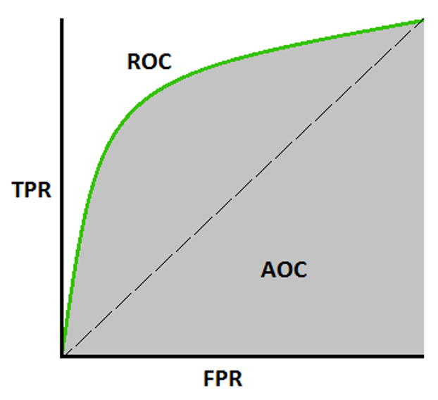
- example
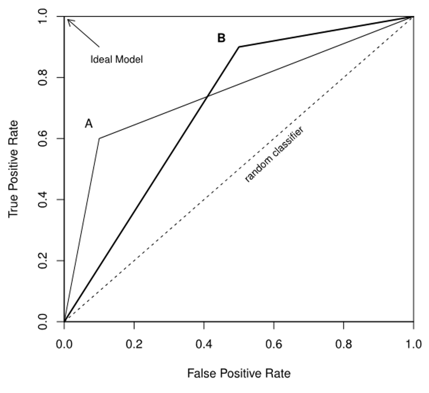
- AUC is always between 0 and 1
- calculate the area of the curve and compare which one is better
- AUC = 1 = ideal situation where all fraud and no fraud cases are correctly predicted
- AUC = 0.5 (i.e. diagonal curve) = random guesses, i.e. no discrimination power between fraud and no fraud cases
- any curves under the diagonal curve = no use
- basic terms
any measures that are applicable for the model developed
- statistics measure
regression model
- MAE (Mean Absolute Error)
- \(y_i\) is the actual expected output and \(\hat{y_i}\) is the model's prediction
- simplest but not popular
\[MAE=\frac{1}{N} \displaystyle \sum^{N}_{i=1} |y_i - \hat{y_i}|\]
- MSE (Mean Squared Error)
- more sensitive to outliers, compared with MAE
\[MSE=\frac{1}{N} \displaystyle \sum^{N}_{i=1} {(y_i - \hat{y_i})}^2\]
- RMSE (Root Mean Squared Error)
- due to squared error terms in MSE
\[RMSE=\sqrt{\frac{1}{N} \displaystyle \sum^{N}_{i=1} {(y_i - \hat{y_i})}^2}\]
- r-squared
- also called coefficient of determination
- explains the degree to which the input variables explain the variation of the output/predicted variable
- limitation: either stay the same or increases with the addition of more variables, even if they do not have any relationship with the output variables
\[R^2=1-\frac{SS_{RES}}{SS_{TOT}}=1-\frac{\sum_i {(y_i-\hat{y_i})}^2}{\sum_i {(y_i-\bar{y})}^2}\]
- adjusted r-squared
- N is the total sample size (number of rows) and p is the number of predictors (number of columns)
- overcome the R-squared limitation
- for building linear regression on multiple variables, suggest to use this method to judge
- but for only one input variable, r-squared and adjusted r-squared are same
\[Adjusted \ R^2=1-\frac{(1-R^2)(N-1)}{N-p-1}\]
scatter plot
- the more the plot approximately a straight, the better the performance of the regression model
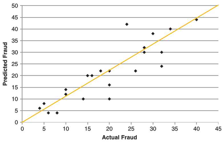
- the more the plot approximately a straight, the better the performance of the regression model
Pearson correlation coefficient
- varies between -1 and +1
- closer to +1 indicates better agreement
\[corr(\hat{y},y)=\frac{\sum^n_{i=1}(\hat{y_i}-\bar{\hat{y}})(y_i-\bar{y})}{\sqrt{\sum^n_{i=1}{(\hat{y_i}-\bar{\hat{y}})}^2}\sqrt{\sum^n_{i=1}{(y_i-\bar{y})}^2}}\]
- MAE (Mean Absolute Error)
comparison
- for classfication model
- the output is categorical data
- the measure of the performance is counting the % of correctly predicted value
for regression model
- the outout is a continuous number
- the measure of the performance is how "close" the predicted value is to the actual value, any deviation from the actual value is an error
\[Error=Y(actual)-Y(predicted)\]
- for classfication model