12 minutes
FITE7410 Financial Fraud Analytics Techniques (Part 2)
.png)
Clustering
Basics about clustering
- aim
- group a set of observations into groups (or clusters)
- feature
- the homogeneity (similarity) within the cluster is maximized
- the heterogeneity (dissimilarity) between the cluster is maximized
- unsupervised classification (no labels)
- no predefined target class
- number of clusters unknown
- meaning of clusters unknown
distance metrics
- measure the similarity and dissimilarity between observations in a group
types
metrics for continuous variables
Minkowski distance
- formula
- \(n\) represents the number of variables
- \(x_i, x_j\) are two observations
\[D(x_i:x_j)={(\sum_{k=1}^n {|x_{ik}-x_{jk}|}^p)}^{1/p}\]
- when p = 1, it is Manhattan (or city block) distance
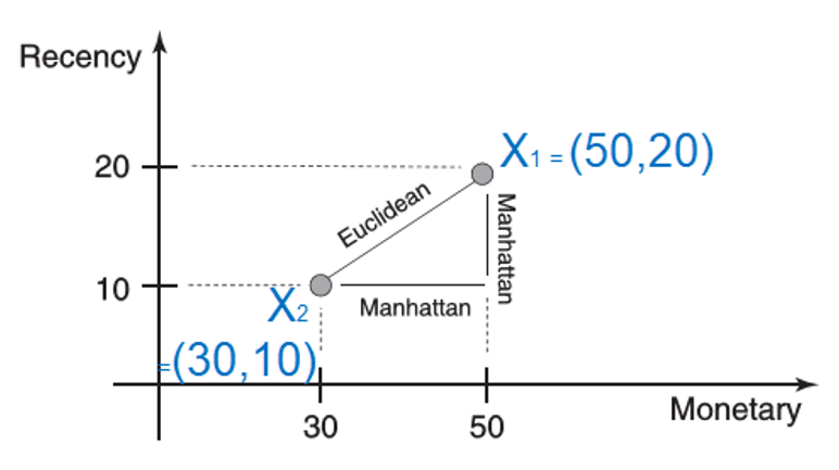
\[D(x_i:x_j)=|x_{11}-x_{21}|+|x_{12}-x_{22}|=|50-30|+|20-10|=30\]
- when p = 2, it is Euclidean distance
\[D(x_i:x_j)=\sqrt{{(x_{11}-x_{21})}^2+{(x_{12}-x_{22})}^2}=\sqrt{{(50-30)}^2+{(20-10)}^2}=22\]
- formula
Pearson correlation
metrics for categorical variables
- simple matching coefficient (SMC)
- calculates the number of identical matches between the variable values
- assumption of SMC is that "Yes" and "No" are of equal weights
- Jaccard index
- similar to SMC, but left out the "No-No" match
- measures the similarity between observations across those red flags that were raised at least once
- especially useful in situations where many red-flag indicators are available and typically only a few are raised
- example
- SMC(Claim1, Claim2) = 2/5
- Jaccard(Claim1, Claim2) = 1/4

- simple matching coefficient (SMC)
Types of clustering
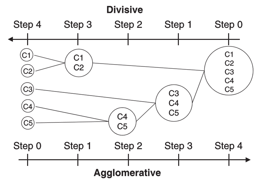
hierarchical
- agglomerative
- bottom-up
- divisive
- top-down
- top-down
- use a similarity or distance matrix to merge or split one cluster at a time
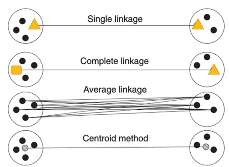
distance matrics
- single linkage: smallest possible distance
- thin, long and elongated clusters since dissimilar objects are not accounted for
- complete linkage: biggest possible distance
- cluster are tight, more balanced and spherical
- average linkage: average of all possible distances
- merge clusters with small variances, results in clusters with similar variance
- centroid method: distance between the centroids of both clusters
- most robust to outliers, but not perform as well as Ward's method or average linkage
- most robust to outliers, but not perform as well as Ward's method or average linkage
Ward's distance: the dendrogram and hierarchy is clearer
- merge clusters with a small number of observations and results in balanced clusters
- formula
\[D_{Ward}(C_i,C_j)=\sum_{x\in C_i}{(x-c_i)}^2+\sum_{x\in C_j}{(x-c_j)}^2-\sum_{x\in C_{ij}}{(x-c_{ij})}^2\]
- find the optimal clustering thru
- dendrogram - termination condition to cut the dendrogram
- screen plot - elbow point indicates the optimal clustering

- single linkage: smallest possible distance
advantages
- easy to interpret and understand (dendrogram is easy to understand)
- relatively easy to implement
- number of clusters does not need to be specified prior to the analysis
disadvantages
- the methods do not scale very well to large data sets, i.e. computationally expansive
- interpretation of clusters is often subjective and depends on expert knowledge
- does not work well with mixed data types and missing data
- not the best solution for data sets with high dimensions
- agglomerative
non-hierarchical
- k-means
- some basics
- k means each cluster is represented by the center (or mean) of the cluster
- need to be specified before the start of analysis
- procedure
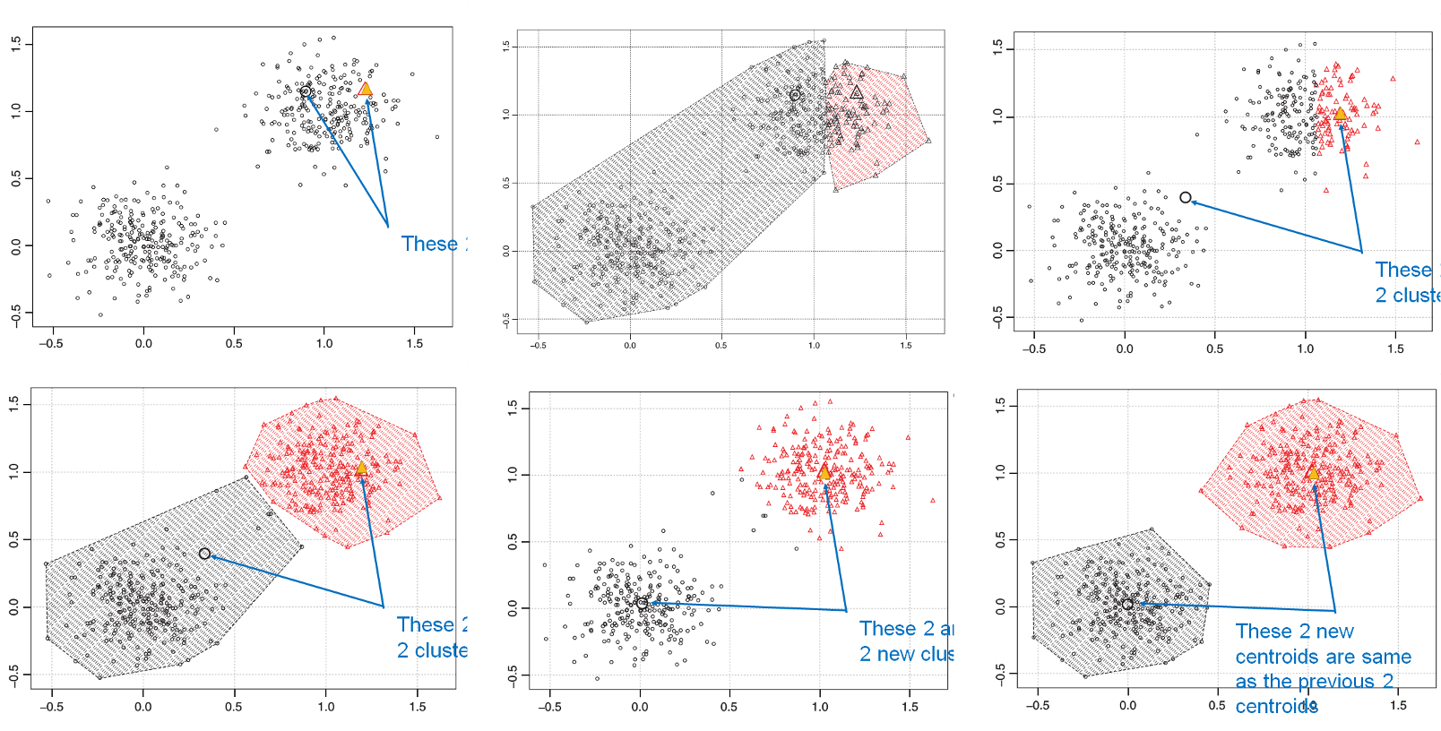
- select k observations as initial cluster centroids (seeds)
- assign each observation to the cluster that has the closest centroid
- when all observations have been assigned, recalculate the positions of the k centroids
- repeat until the cluster centroids no longer change or a fixed number of iterations is reached
- advantages
- relatively computational efficient as compared with hierarchical clustering
- simple to implement and scales to large datasets
- disadvantages
- need to specify k, the number of clusters, in advance
- often terminates at a local optimum, need to try different initial cluster centres
- unable to handle noisy data and outliers
- some basics
- self-organizing map (SOM)
- k-means
many others
- density-based
- model-based
- graph-based
Performance Evaluation of Clustering
Overivew
- method
- no universal criterion for clustering performance evaluation
- only 2 perspectives
- statistical perspective
- interpretability perspective
- the standard of a good clustering solution
- high within-cluster similarity
- low between-cluster similarity
SSE (Sum of Square Error)
- a statistical method
- how to evaluate
- the lower the SSE for a particular cluster (WSS), the more homogenous is that cluster, i.e. higher within-cluster similarity
- the higher the SSE among different clusters (BSS), the more heterogenous are the clusters, i.e. lower between-cluster similarity
- the optimal number of clusters
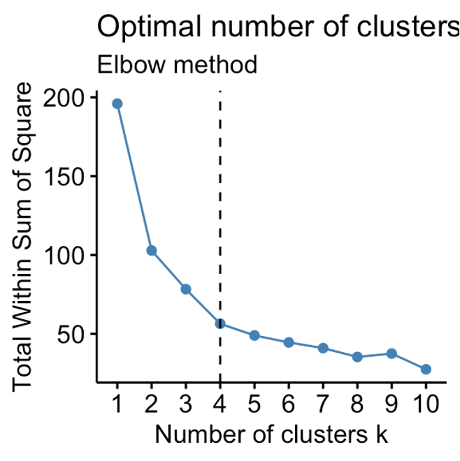
- elbow method - makes use of within-cluster SSE (WSS)
- steps
- compute the k-means clustering models for different k values
- for each k, calculate the WSS
- plot WSS accoriding to the value of k
- find the point where there is a bend (or elbow) in the curve -> optimal
Interpretation of a clustering solution
- compare clusters with population distribution (or between clusters)
- plot histogram, mean, bar charts etc of those most important variables by clusters
- example
- cluster C1 has observations with low recency values and high monetary values, whereas the frequency is similar to original population

- cluster C1 has observations with low recency values and high monetary values, whereas the frequency is similar to original population
- use classification tree
- to predict the target variables
- example

Neural Network
Basic concepts
- neural networks (NN)
- can be used to perform tasks like classification, clustering, predictive analytics
- ANN & DNN
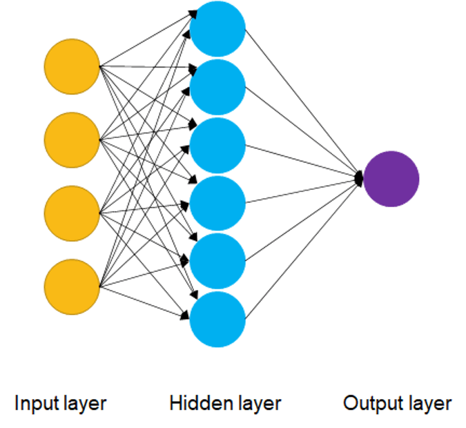
- artificial neural networks (ANN) are composed of layers of node/neurons
- neural networks with more than one hidden layer are called deep neural networks (DNN)
- structure
- input layer - initial input data for the neural network (visible layer)
- hidden layers - between input and output layers, where the computations are done and passed on to other nodes deeper in the neural network
- output layer - output result of the given input (visible layer)
Inside an artificial neuron
- activation functions
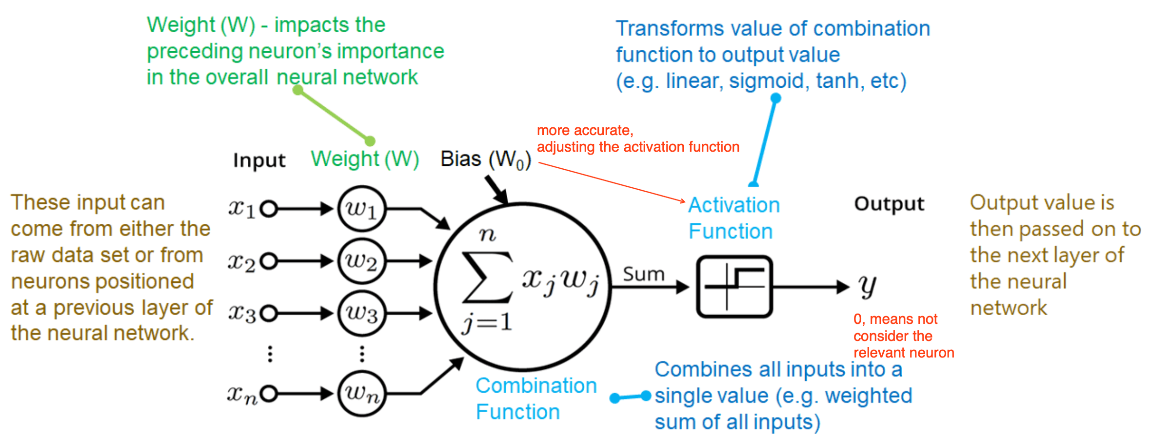
- mathematical equations that determine the output of a neural network
- attached to each node and defines if the given node should be “activated”, based on whether each node’s input is relevant for the model’s prediction
- normalize the output of each neuron to a range between 1 and 0 or between -1 and 1
- examples
- linear activation functions
- threshold (unit step or sign) function
- only classify output as 0 or 1
- linear function
- transform the output of the neural network into a linear function, unable to cater for non-linear data

- transform the output of the neural network into a linear function, unable to cater for non-linear data
- threshold (unit step or sign) function
- non-linear activation functions (most neural networks use this for more complex mappings between inputs and outputs)
- Sigmoid function
- can accept any value and normalize output between 0 to 1
- smooth gradient and clear predictions
- problems
- output not zero centered & computationally expensive
- vanishing gradient - when the sigmoid function value is either too high or too low, the derivative becomes very small i.e. << 1, causing poor learning for deep networks
- TanH (hyperbolic tangent) function
- similar to Sigmoid function, but zero centered, i.e. easier to model inputs with strong negative, neutral and positive values
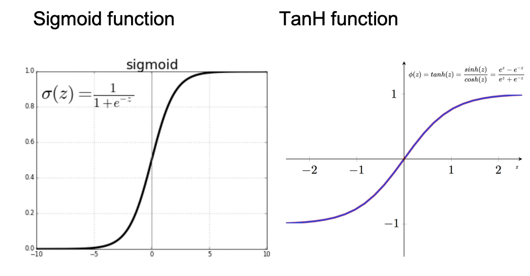
- similar to Sigmoid function, but zero centered, i.e. easier to model inputs with strong negative, neutral and positive values
- Sigmoid function
- linear activation functions
Training a neural network
cost/loss function
- NN is trained based on this
- to measure the error of the network's prediction, or how good the neural network model is for a particular task
cost function - MSE
- difference between predicted output and actual output
- square the difference and
- calculate the mean
\[MSE=\frac{1}{n}\sum_{i=1}^n{(Y_i-\hat{Y_i})}^2\]
MSE should be as small number as possible
process

for fraud analytics
- usually one hidden layer is enough
- theoretically can use different activation function at each node, but usually this is fixed for each layer
- for hidden layers (black-box approach)
- use non-linear functions, e.g. TanH function
- for output layers
- classification targets (fraud vs non-fraud): use sigmoid function
- regression target (e.g. amount of fraud): can use any function
- data pre-processing
- normalize the continuous variables, e.g. using z-scores
- reduce the number of categories for categorical variables
Interpret neural network
- variable selection
- features
- to select those variables that actively contribute to the neural network output
- does not give insight about the internal workings of the neural network
- Hinton diagram
- visualizes the weights between inputs and hidden neurons as squares
- size of square is proportional to size of the weight
- color of the square represents sign of the weight (e.g. black = -ve, white = +ve)
- e.g. “Income” variable can be removed
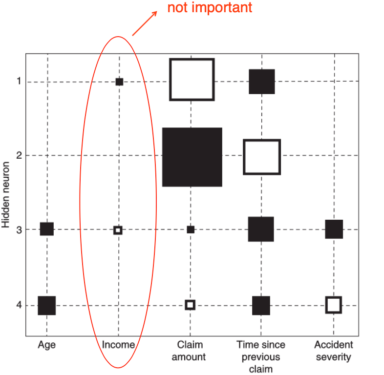
- variable selection procedures
- inspect the Hinton diagram and remove the variable whose weights are closest to ZERO
- re-estimate the neural network with the variable removed (to speed up the convergence, it could be beneficial to start from the previous weights)
- continue with step 1 until a stopping criterion is met, the stopping criterion could be a decrease of predictive performance or a fixed number of steps
- backward variable selection procedures
- build a neural network with all N variables
- remove each variable in turn and re-estimate the network (this will give N networks each having N-1 variables)
- remove the variable whose absence gives the best performing network (e.g. in terms of misclassification error, mean squared error)
- repeat this procedure until the performance decreases significantly
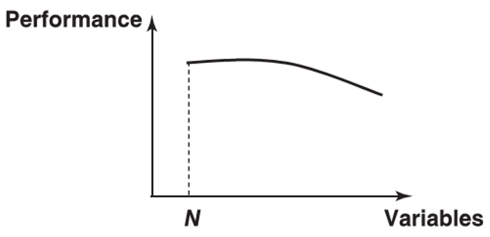
- features
- rule extraction
- feature
- extract if-then classification rules
- decompositional approach
- decompose the network’s internal workings by inspecting weights and/or activation values
- example
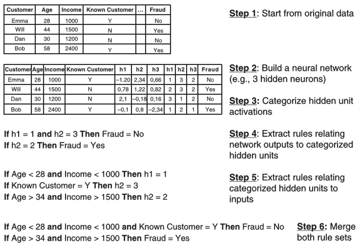
- pedagogical approach
- example
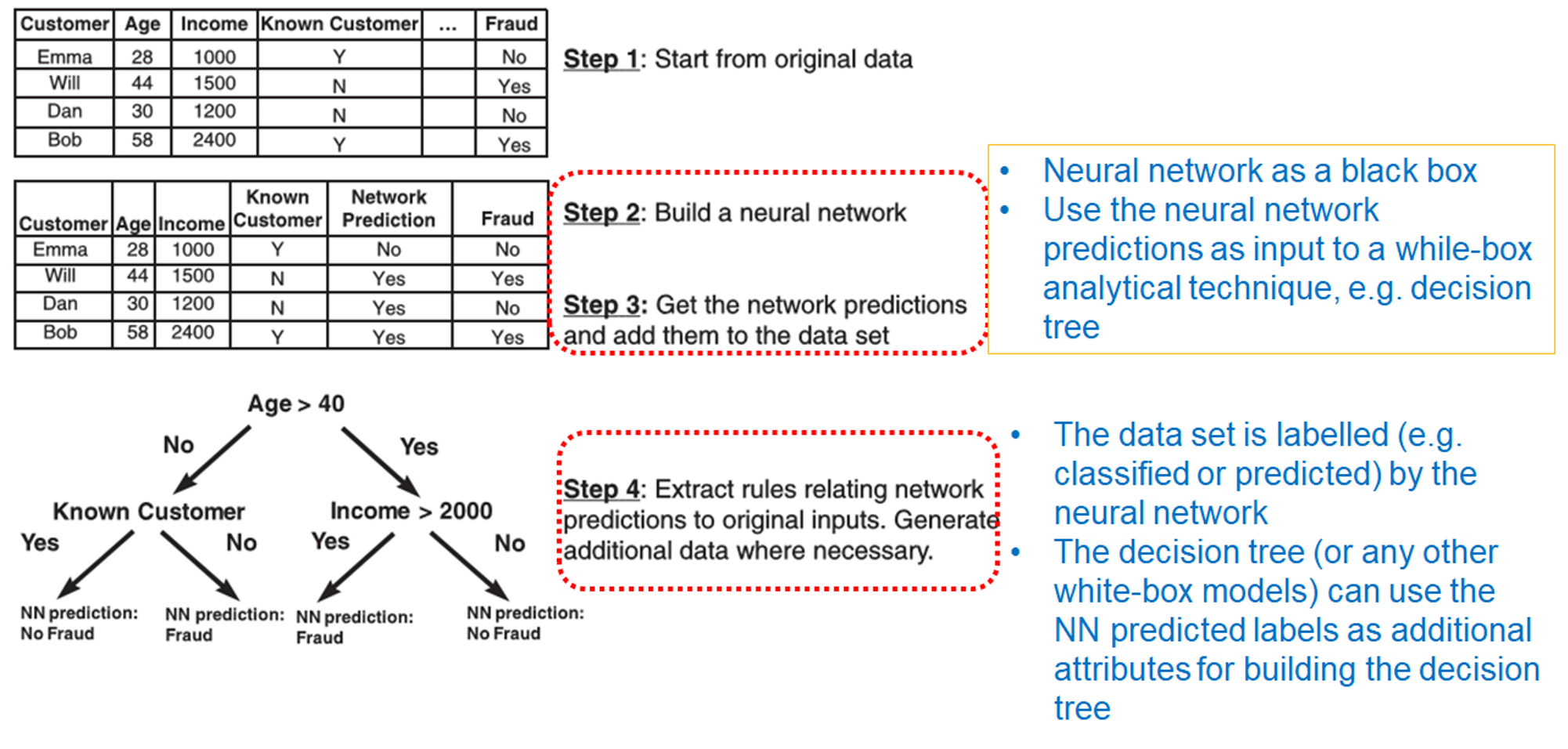
- example
- performance evaluation
- rules extraction sets evaluated in terms of
- accuracy
- conciseness (e.g. number of rules, number of conditions per rule)
- fidelity – measures to what extent the extracted rule set succeeds in mimicking the neural network

- benchmark the extracted rules/trees with a tree built directly on the original data to see the benefit of going through the neural network
- rules extraction sets evaluated in terms of
- feature
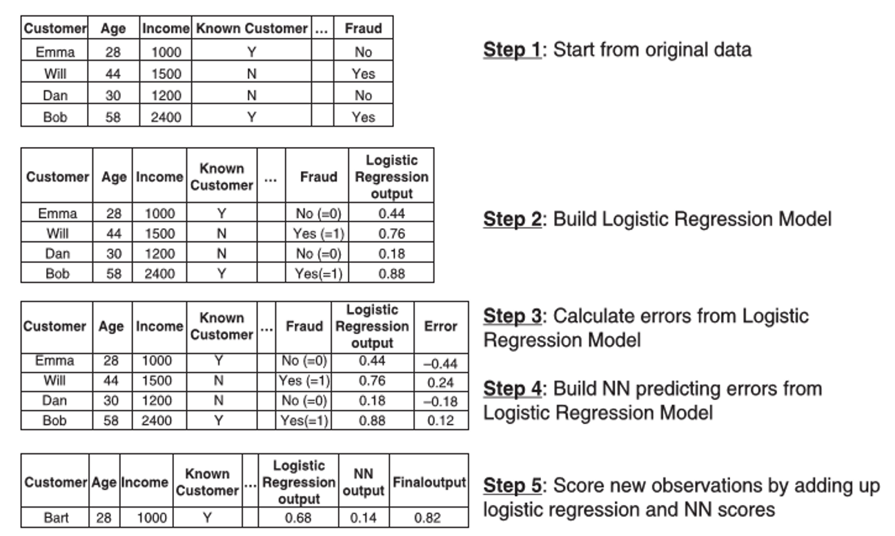
- two-stage models
- combines 2 models with both interpretability and performance
- procedure
- stage 1 (model interpretability)
- to estimate an easy-to-understand model (e.g. linear regression, logistic regression)
- stage 2 (model performance)
- to predict the errors made by the simple model using the same set of predictors
- stage 1 (model interpretability)
- example
Advantages and disadvantages
- advantages
- handle different types of input variables and support multivariate targets
- support flexible and nonlinear relations between input and target variables
- due to flexibility of the model, it is applicable to many problems
- disadvantages
- black-box model, not easy to interpret
- prone to overfit
- requires handling of input attributes, e.g. data imputation
Support Vector Machine (SVM)
Overview
- issues with NN
- the objective function is nonconvex (i.e. may have multiple local minima)
- the effort needed to tune the number of hidden neurons
- basics of SVM
- supervised learning model that can be used for both classification and regression tasks
- more commonly used for classification tasks
- basic idea - to find a line or a hyperplane that best divides the dataset into 2 classes
Basic idea
- linear classification
- decision boundary
- 1-d: a dot
- 2-d: a line
- n-d: hyperplane
- steps
- find the points (support vector) that are closest to the hyperplane (the line) from both classes
- compute the margin = distance between the support vectors and hyperplane
- find the hyperplane with the maximal margins
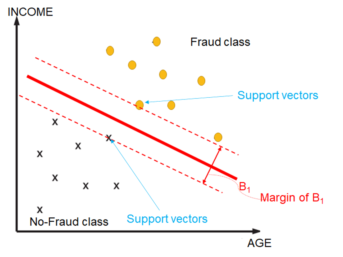
- objective of SVM
- to maximize margins between the two dotted lines
- i.e. the 2 classes are far away as possible
- linear nonseparable
- introduce some values
- error term (\(e_k\)) allows for misclassification errors
- hyperparameter (C) balances importance maximizing the margin or minimizing the error of on the data
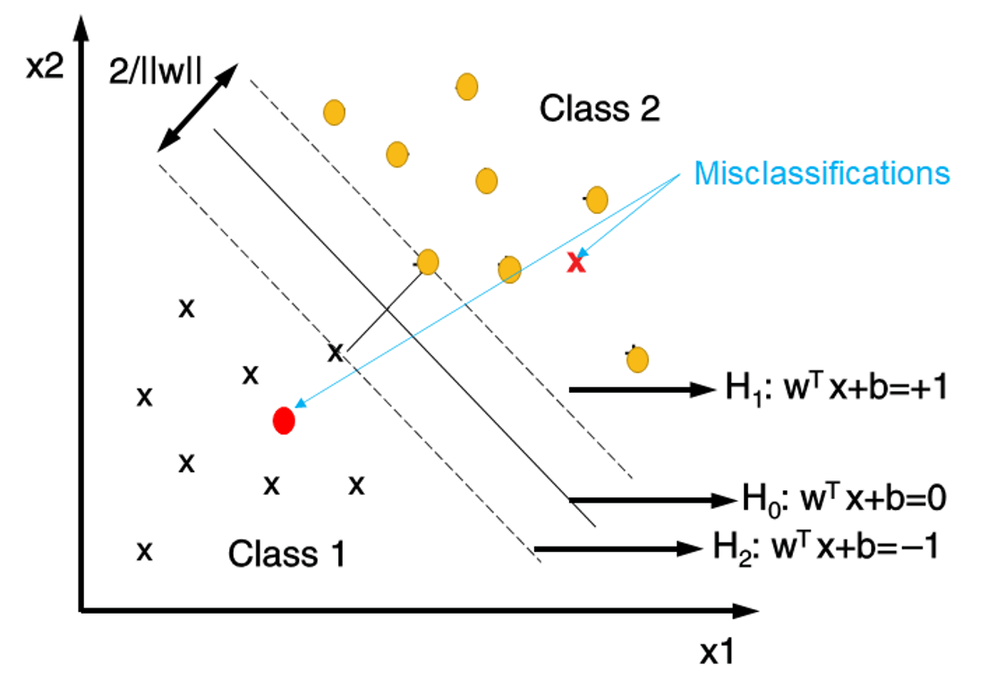
- if it is linear separable, just ignore the above values
- introduce some values
- decision boundary
nonlinear classification
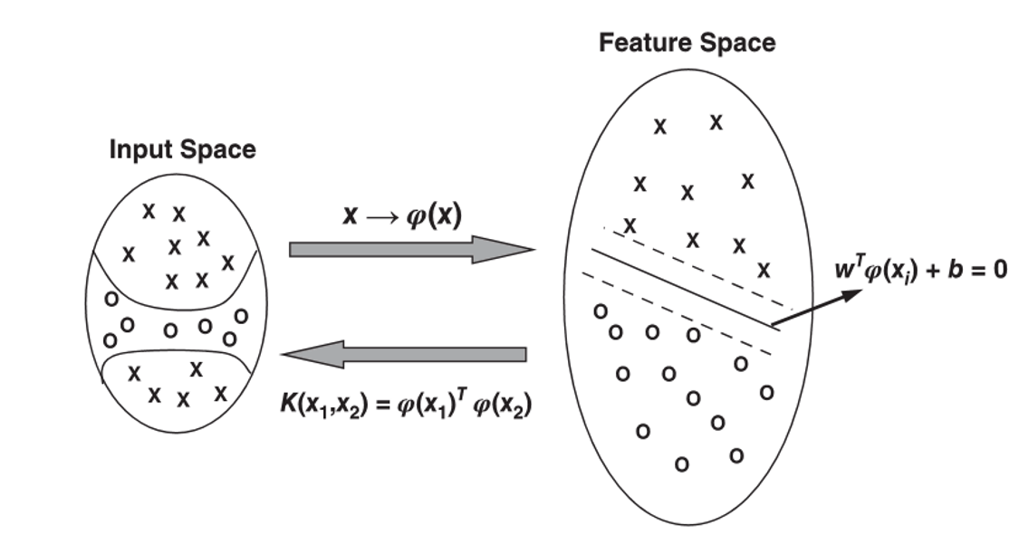
mapping function \(\phi(x)\)
- transform the input data points to a higher dimensional feature space
- mathematically, it is not needed (need kernel function actually)
kernel trick
- formula
\[K(x_k,x_l)=\phi(x_k)^T\phi(x_l)\]
- formula
commonly used kernel functions
- linear kernel: \(K(x,x_k)=x_k^Tx\)
- polynomial kernel: \(K(x,x_k)={(1+x_k^Tx)}^d\)
- radial basis function (RBF) kernel: \(K(x,x_k)=exp\{-{||x-x_k||}^2/\sigma^2\}\)
- example
- RBF kernel usually performs best, but you need to tune the extra parameter gamma \(\sigma\)

- RBF kernel usually performs best, but you need to tune the extra parameter gamma \(\sigma\)
tuning of hyperparameters
- hyperparameter C - penalty parameter representing an error or any form of misclassification
- small C value
- hyperplane with a larger margin, i.e. more violations are allowed, maximizing the margins
- large C value
- hyperplane with a tighter margin, i.e. more emphasis is placed on minimizing the number of classifications

- hyperplane with a tighter margin, i.e. more emphasis is placed on minimizing the number of classifications
- just try to balance, which one should be used, thinking about the performance
- small C value
- gamma
- only need to tune this hyperparameter if you use nonlinear hyperplane
- lower value of gamma
- create a loose fit of the training dataset
- consider only the nearby points for the calculation of a separate plane
- higher value of gamma
- tries to exactly fit the training data
- consider all the data-points to calculate the final separation line
- which one is better, defined by performance (each one is good, the difference is boundary)

procedure
- partition the data into 40%, 30%, 30% training, validation and test data
build an RBF SVM classifier for each (\(\sigma, C\))
\[\sigma \in \{0.5, 5, 10, 15, 25, 50, 100, 250, 500\}\]
\[C \in \{0.01, 0.05, 0.1, 0.5, 1, 5, 10, 50, 100, 500\}\]
choose the (\(\sigma, C\)) combination with the best validation set performance
build an RBF SVM classifier with the optimal (\(\sigma, C\)) combination on combined training + validation dataset
calculate the performance of the estimated RBF SVM classifier on the test set
- hyperparameter C - penalty parameter representing an error or any form of misclassification
SVM interpretation
- SVM classifier can be presented as a neural network
- then, use the techniques in neural network interpretation
- SVM prediction -> decision tree (like previous example)
Advantages and disadvantages
- advantages
- works really well with a clear margin of separation
- effective in high dimensional spaces and where the number of dimensions is greater than the number of samples
- uses a subset of training points in the decision function (called support vectors), so it is also memory efficient
- disadvantages
- does not perform well when data set is large, and when the data set has more noise
- choosing the effective kernel function can be computationally intensive
Multiclass Classification Techniques
Binary vs multiclass
- binary
- label as "fraud" and "no fraud"
- multiclass
- more than 2 labels
- nominal labels
- fraud, suspected fraud, no fraud
- ordinal labels
- severe fraud, medium fraud, light fraud, no fraud
- severe fraud, medium fraud, light fraud, no fraud
Techniques
logistic regression (for nominal target variables)
choose one of the target class (e.g. class K) as the base class
\[\frac{P(Y=1|X_1,\ldots,X_N)}{P(Y=K|X_1,\ldots,X_N)}=e^{(\beta_0^1+\beta_1^1X_1+\beta_2^2X_2+\ldots+\beta_N^1X_N)}\]
\[\frac{P(Y=2|X_1,\ldots,X_N)}{P(Y=K|X_1,\ldots,X_N)}=e^{(\beta_0^2+\beta_1^2X_1+\beta_2^2X_2+\ldots+\beta_N^2X_N)}\]
\[\cdots\]
\[\frac{P(Y=K-1|X_1,\ldots,X_N)}{P(Y=K|X_1,\ldots,X_N)}=e^{(\beta_0^{K-1}+\beta_1^{K-1}X_1+\beta_2^{K-1}X_2+\ldots+\beta_N^{K-1}X_N)}\]
based on the fact that all probabilities sum to 1
\[P(Y=1|X_1,\ldots,X_N)=\frac{e^{(\beta_0^1+\beta_1^1X_1+\beta_2^2X_2+\ldots+\beta_N^1X_N)}}{1+\sum_{k=1}^{K-1}e^{(\beta_0^k+\beta_1^kX_1+\beta_2^kX_2+\ldots+\beta_N^kX_N)}}\]
\[P(Y=2|X_1,\ldots,X_N)=\frac{e^{(\beta_0^2+\beta_1^2X_1+\beta_2^2X_2+\ldots+\beta_N^2X_N)}}{1+\sum_{k=1}^{K-1}e^{(\beta_0^k+\beta_1^kX_1+\beta_2^kX_2+\ldots+\beta_N^kX_N)}}\]
\[P(Y=K|X_1,\ldots,X_N)=\frac{1}{1+\sum_{k=1}^{K-1}e^{(\beta_0^k+\beta_1^kX_1+\beta_2^kX_2+\ldots+\beta_N^kX_N)}}\]
parameter \(\beta\) is estimated using maximum aposteriori estimation, which is extension of maximum likelihood estimation
decision tree
the impurity criteria can be written as follows (K is the number of class labels)
\[Entropy(S)=-\displaystyle \sum^K_{k=1}p_klog_2(p_k)\]
\[Gini(S)=\displaystyle \sum^K_{k=1}p_k(1-p_k)\]
the splitting and stopping decisions are the same as the binary class classifications
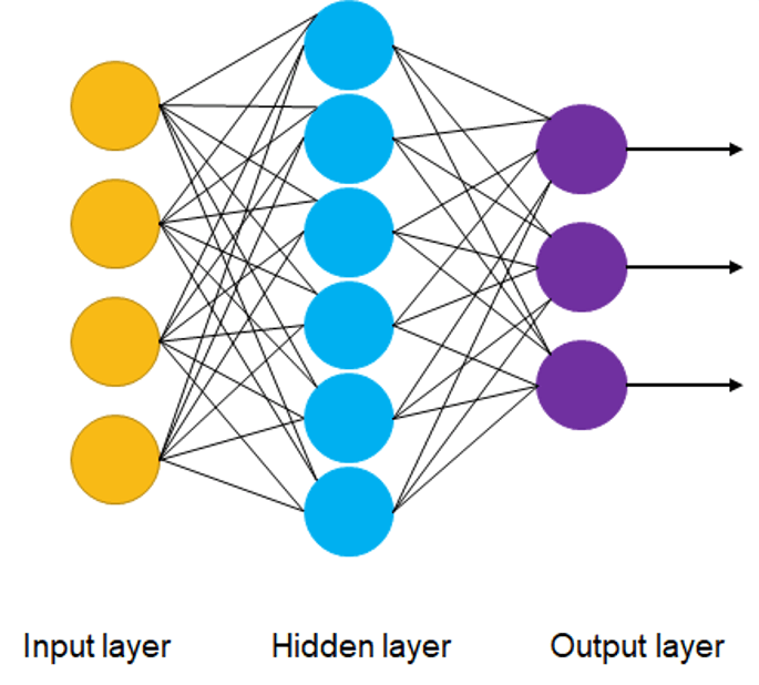
NN
- increase the number of output neurons to K, where K corresponds to K class labels
- an observation is assigned to the output neuron with the highest activation value
SVM
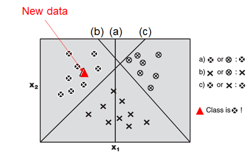
- treat is as binary class problem by dividing the target classes into 2 classes
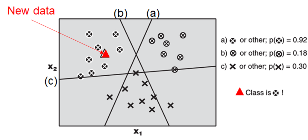
- one-versus-one, for a K target classes, learn K SVMs as follows
- classifies target as "y=1" vs "y=2"; "y=1" vs "y=3"; ... "y=1" vs "y=K"; "y=2" vs "y=3"; "y=2" vs "y=4"; ... "y=2" vs "y=K" ...
- will have \(\frac{K(K-1)}{2}\) classifiers
- use a (weighted) voting procedure for the final classification result
- one-versus-all, for a K target classes, learn K SVMs as follows
- SVM#1, with target class label=1, classifies target as “y=1” vs “y≠1"
- SVM#2, with target class label=2, classifies target as “y=2” vs “y≠2"
- SVM#K, with target class label=K, classifies target as “y=K” vs “y≠K”
- use the highest posterior probability to decide the classification result
