pre-process the raw data before proceeding to conduct the analysis steps
Data sources
types
structured
transactional data
contractual, subscription, or account data
surveys
behavoural information
unstructured
text documents, e.g. emails, web pages, claim forms or multimedia contents
contextual or network information
qualitative expert-based data
publicly available data
semi-structured
5Vs
velocity
volume
variety
veracity
value
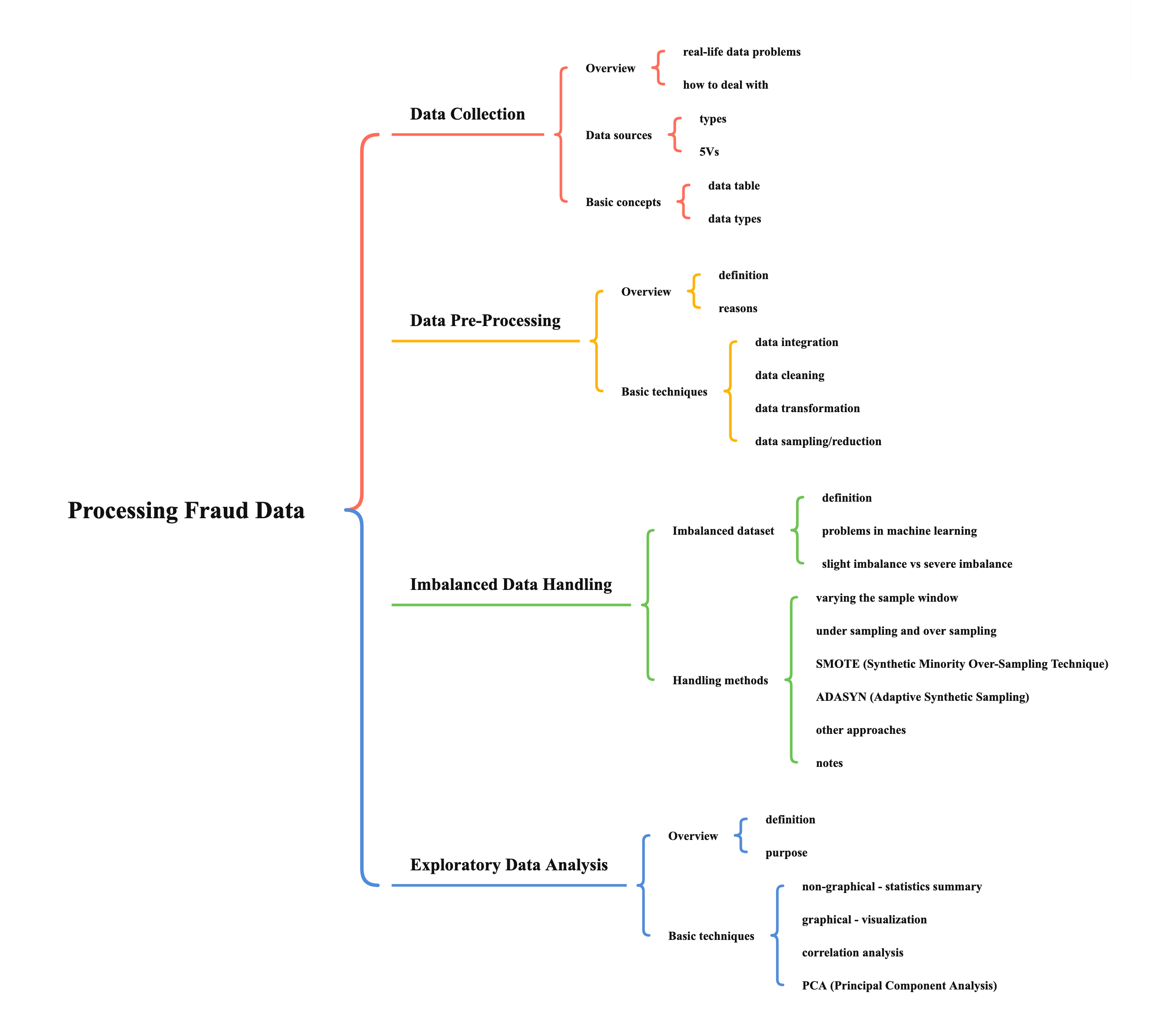
Basic concepts
data table
columns, variables, fields, characteristics, attributes, features, etc. -> same things
rows, instances, observations, lines, records, tuples, etc. -> same things
data types
continuous data
e.g. amount of transactions, balance on saving account, similarity index
categorical data
nominal
e.g. marital status, payment type, country of region
ordinal
e.g. age code as young, middle-age, and old
binary
e.g. yes/no, 1/0 (only two values)
Data Pre-Processing
Overview
definition
a process to transform raw data into some usable format for the next data analytics step
provides techniques that can help us to understand and make knowledge discovery of data at the same time
reasons
to deal with the problems of raw data, e.g. noise, incompleteness, inconsistencies
to make sense of the raw data, i.e. to transform raw data into an understandable format
Basic techniques
data integration
combines data from multiple sources into a coherent data store
problems
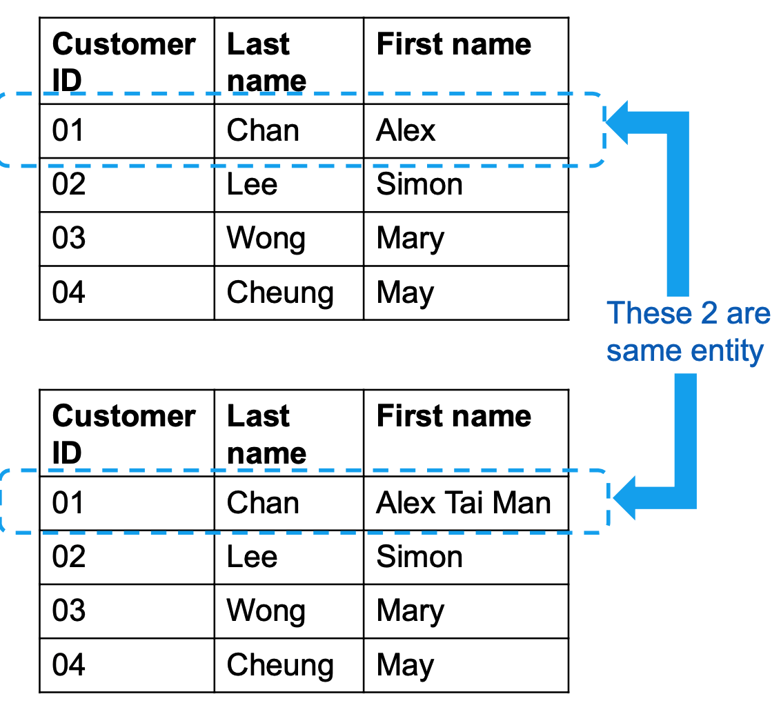
entity identification problem
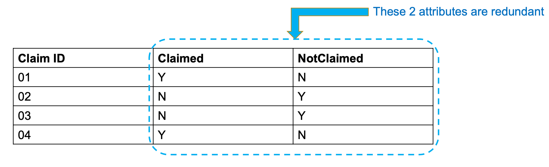
redundant attribute problem
tuple (record) duplication problem
redundant records after merging data from different sources
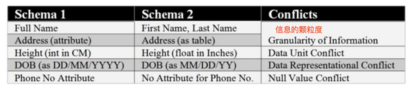
data conflict problem
data cleaning
attempts to fill in missing values (incompleteness), smooth out noise while identifying outliers, and correct inconsistencies in the data
"dirty" data
incomplete/missing data
human input error, intentionally hiding some information
not applicable values, e.g. if there are records without visa card, visa card transactions will be not applicable
not matching search or filter criteria, e.g. if transaction > 1 billion
nosiy data (outliers or errors)
reasons of outliers
valid observations, e.g. salary of senior management > $1M
invalid observations, e.g. age > 300
data inconsistencies (similar to data conflict in data integration)
duplicate records (similar to data duplication in data integration)
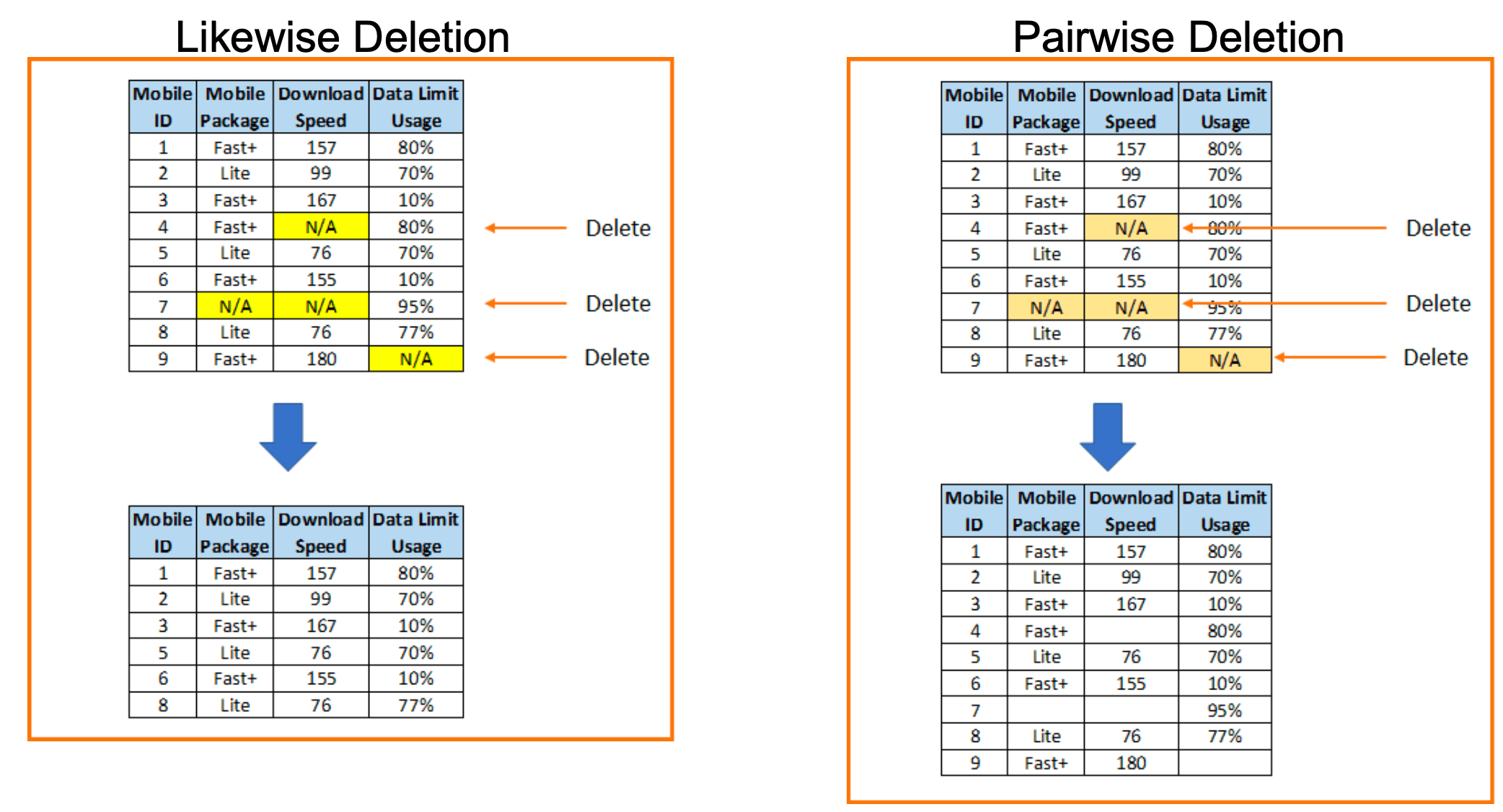
resolution - missing data
listwise/pairwise deletion
problems
listwise - reduced sample size and possibility of missing some important information
pairwise - still have the problem of drawing conclusions based on a subset of data only
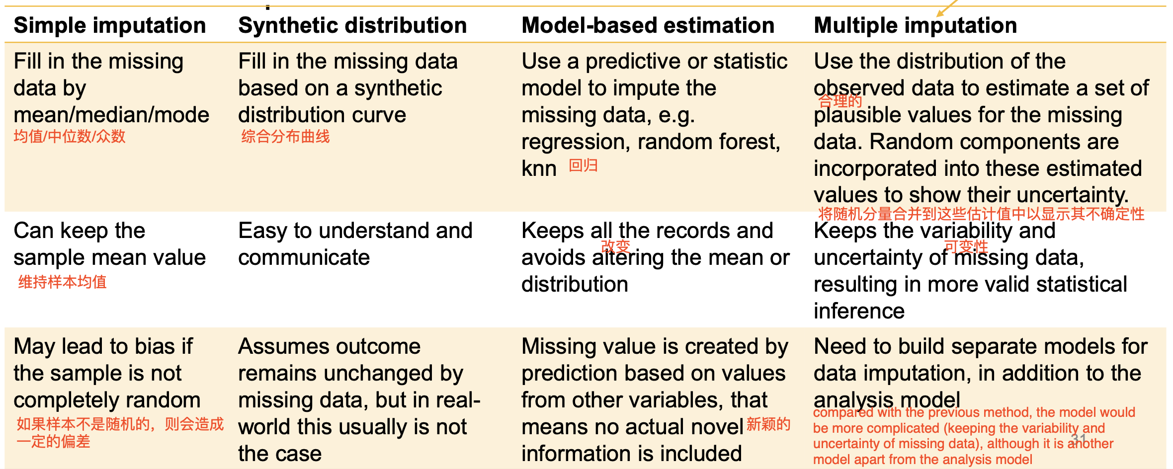
data imputation - fill in the missing data
4 techniques
which method should be used, it really depends on the dataset, the volume of missing data and skill level of various methods
model-based estimation uses one model, if the value of one attribute is lost, it can use the other attributes to estimate the attribute
multiple imputation uses different models and average the results, need to build separate models for data imputation, in addition to the analysis model
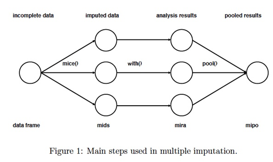
MICE - a packet in R (multiple imputation)
mice()
generate several datasets (normally is 5), stored in mids
these datasets are copies of the original dataframe except that missing values are now replaced with values generated by mice()
with()
run the ols regression on all datasets in mids
obtain a different regression coefficient for each dataset, reflecting the effect of each variable on output
coefficients are different because each dataset contains different imputed values, we do not know which one is correct in advance
the results are stored in mira
pool()
transmit coefficients into one regression coefficient, just take the mean
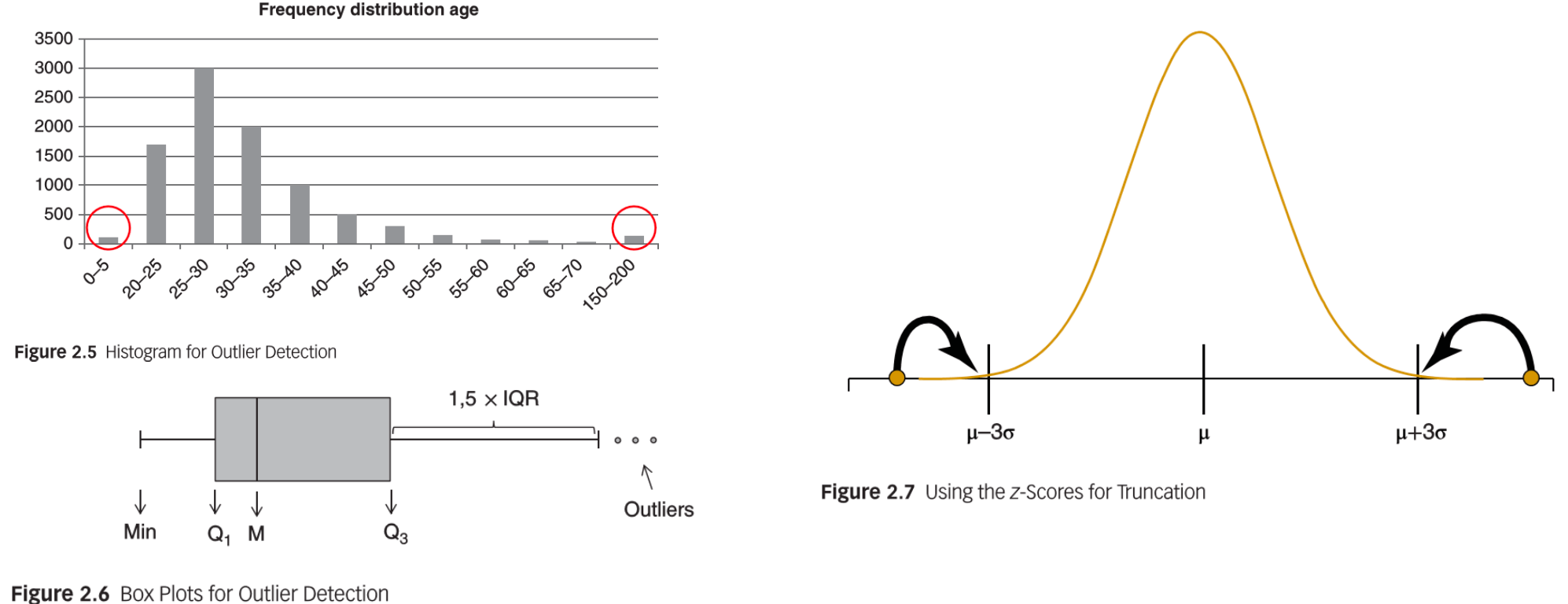
resolution - outliers
detection
calculate minimum, maximum, z-score values for each attribute
define outliers when absolute value of z-score is longer than 3
use visualization, e.g. histogram, box plots
treatment
for invalid observations, treat the outlier as missing value and can use one of the techniques for handling missing value to deal with outlier value
for valid observations, truncation/capping/winsorizing, i.e. set upper and lower limits on a variable
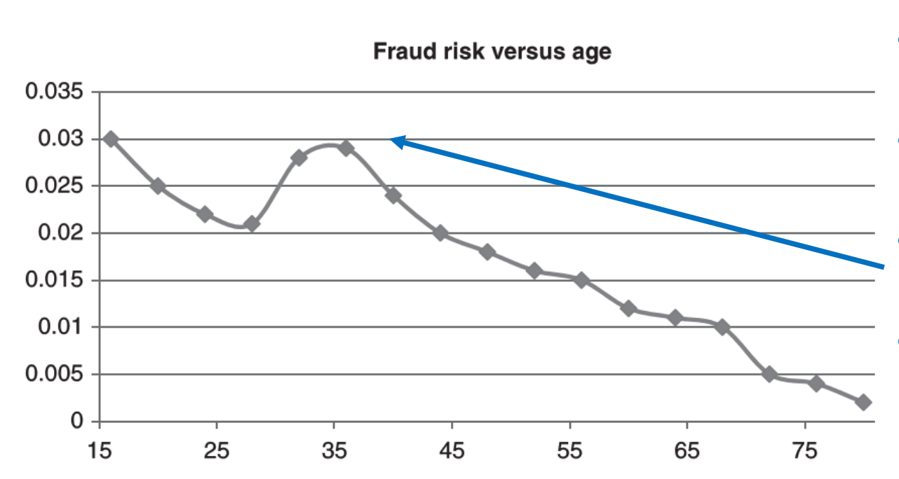
outliers may sometimes be actually the fraud cases, because behaviors of fraudsters usually deviant from normal non-fraudsters
these diviations from normal patterns are red flags of fraud, e.g. small payment followed by a large payment immediately -> may be credit card fraud
caution or mark when deal with outliers -> for further analysis
data transformation
data are transformed into appropriate format for data analysis, also known as ETL (Extract, Transform, Load)
purposes
for easy comparison among different data sets with diverse format
for easy combination with other data sets to provide insights
to perform aggregation of data
techniques
normalization
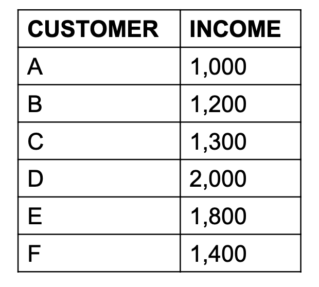
required only when attributes have different ranges
e.g. AGE range from 0 - 100, INCOME range from 10,000 - 100,000 -> INCOME might have larger effect on the predictive power of the model due to its large value
for continuous variables
min-max normalization (range normalization)
z-score standardization
(natual) log or base-10 log
square root
inverse
square
exponential
centring (subtract mean)
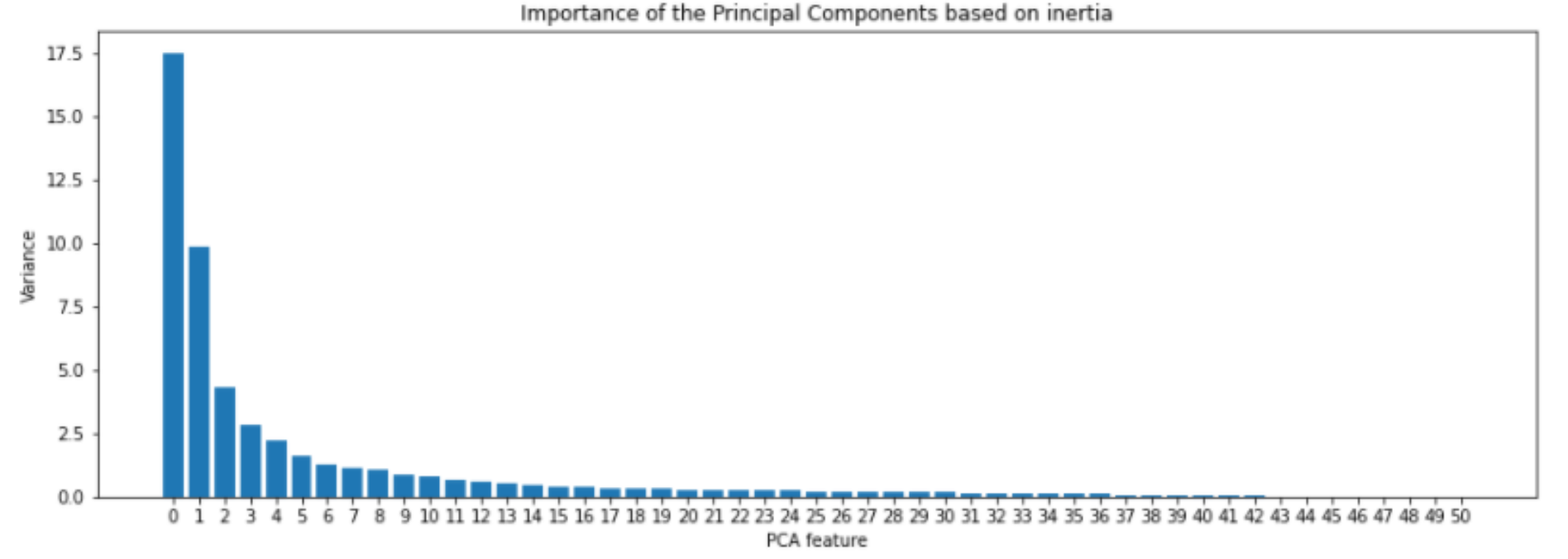
attribute (feature) construction
transform a given set of input features to gnerate a new set of more powerful features
purpose
dimensionality reduction
prediction performance improvement
method - PCA
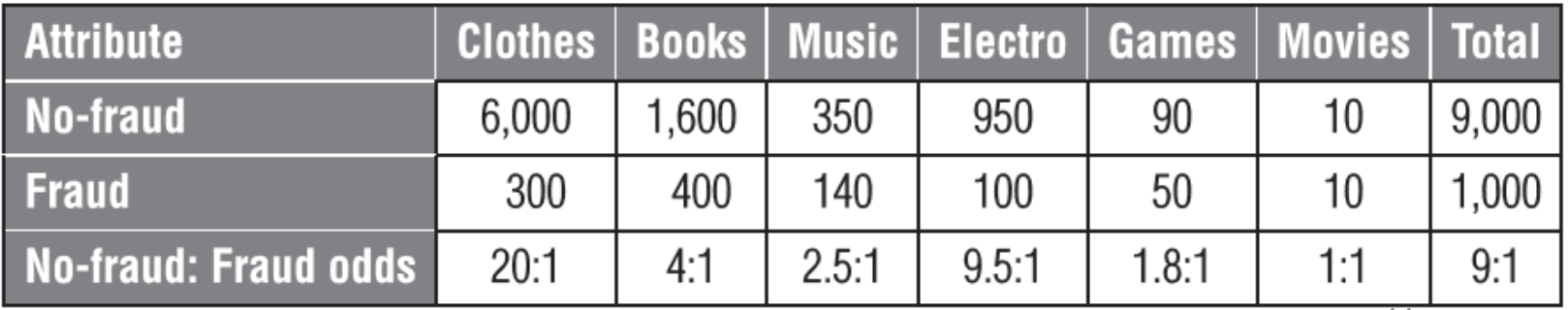
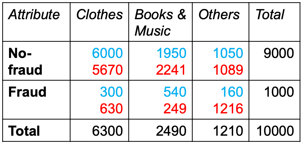
discretization
replace the values of numeric attribute (continuous variable) by conceptual values (discrete variable)
e.g. replace AGE (numeric value) with AGEGROUP (children, youth, adult, elderly), group rare levels into one discrete group "OTHER"
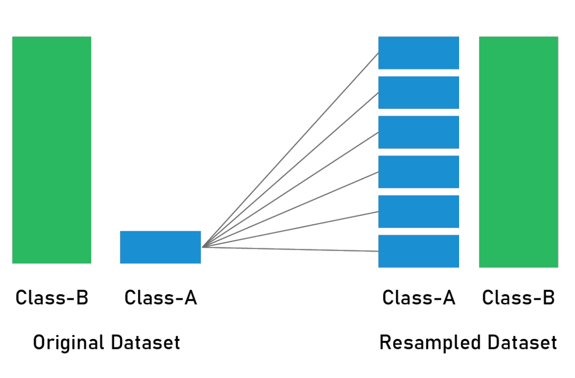
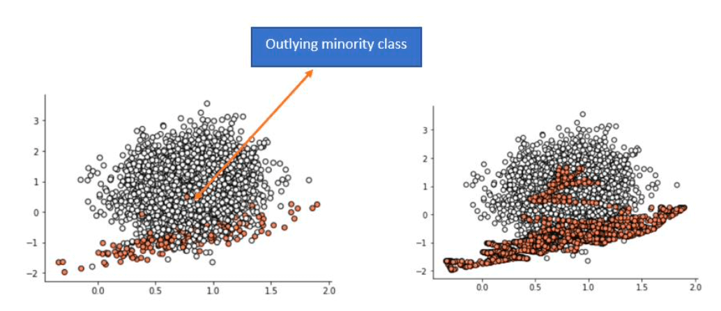
creates synthetic observations based upon the existing minority observations
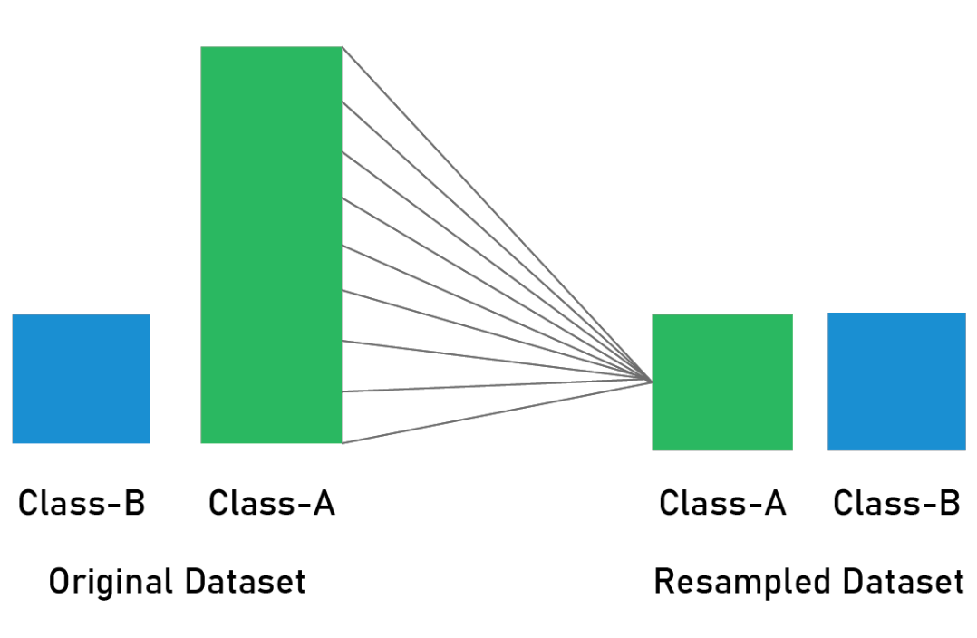
combines the synthetic oversampling of the minority class with undersampling the minority class
is better than either under-/over- sampling, can be used in fraud detection
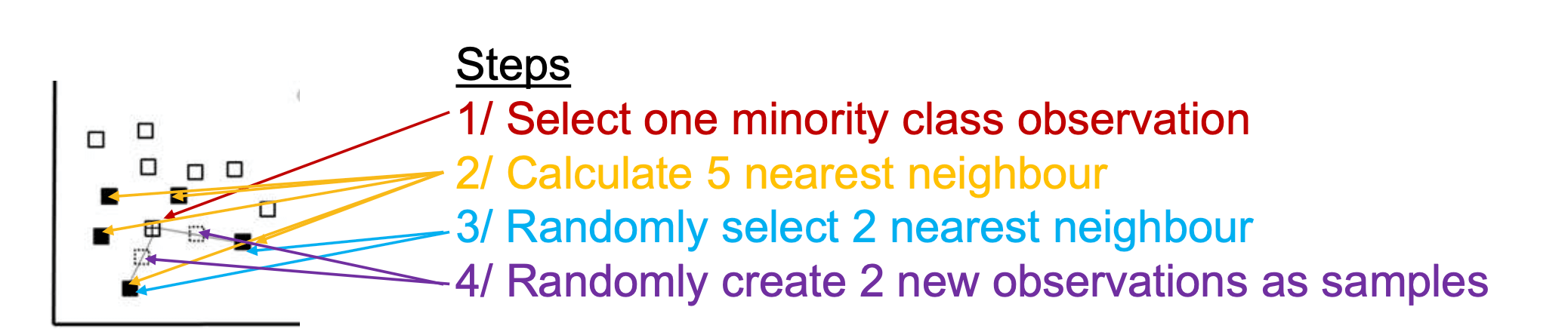
example - select using line
problem
may create a line bridge with the majority class, if the observations in minority class are outlying and appears in majority class
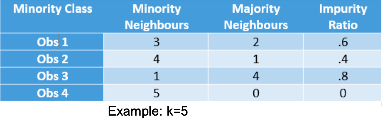
ADASYN (Adaptive Synthetic Sampling)
a generalization of the SMOTE algorithm
takes into account the distribution of density
measures the k-nearest neighbors for all minority instances, then calculates the class ratio of the minority and majority instances to create new samples
impurity ratio is calculated for all minority data points
higher the ratio, more synthetic data points (minority class) are created
example
the synthetic data points of Obs3 will double that of Obs2
other approaches
using probabilities
likelihood approach
adjusting posterior probabilities
cost-sensitive learning - assign higher misclassification costs to minority class (i.e. fraud cases)
notes
the performance of both sampling and cost-sensitive learning approaches are good and equivalent for handling imbalanced dataset
suggest to adopt the sampling approaches for fraud analytics
Exploratory Data Analysis
Overview
definition
the process of using quick and simple methods for the visualization and examination of small data, e.g. boxplots, histograms, etc.
but it is not feasible to use traditional EDA to analyze dataset, due to 5Vs
purpose
to have a better understanding of the data before building the fraud detection model
to detect problems in data
Basic techniques
non-graphical - statistics summary
illustrate relationships between two or more data variables using statistics or cross-tabulation
as a preview to check the symmetry or asymmetry of the distribution, i.e. skewness of the data
calculate for the whole sample set and target set
using descriptive statistics
mean, median (for continuous variables)
mode (for categorical variables)
standard deviation (represent how much data is spread around the mean)
percentile distribution (percentage/distribution of the data)
graphical - visualization
using picture of data, such as stem-and-leaf plots, box plots, pie chart, histogram, scatter plot
missing data, outliers, and distribution can be more easily identified using visualization of the data
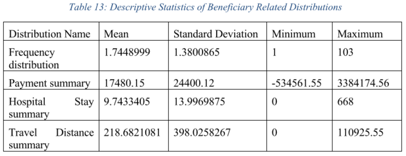
example
the maximum value of hospital stay is 668 (> 365) -> impossible
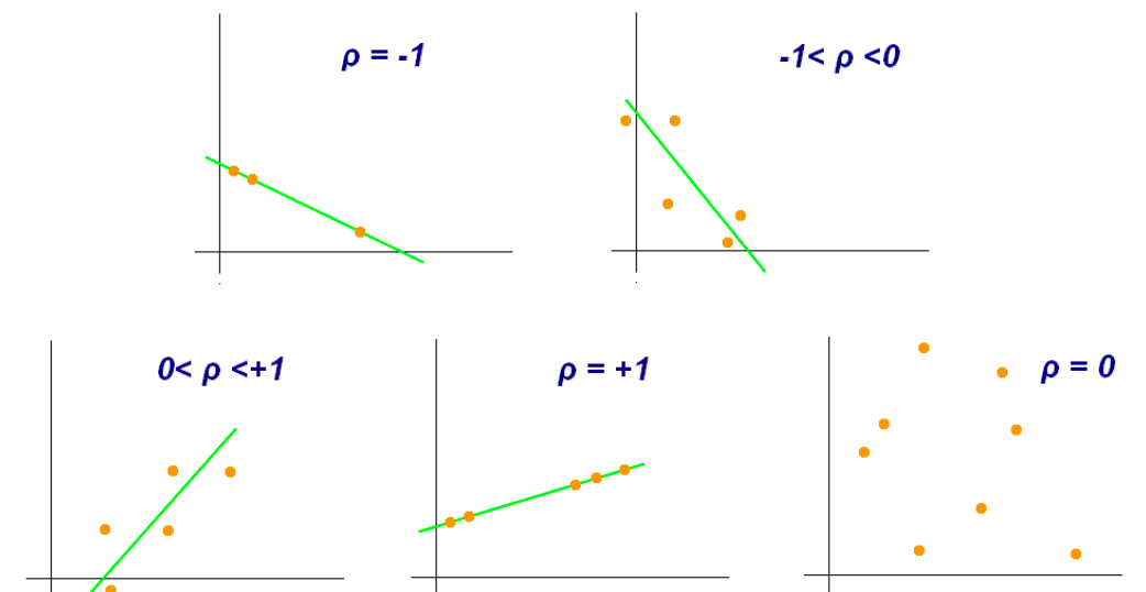
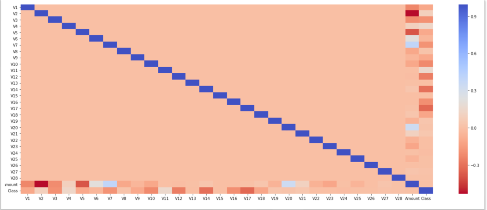
correlation analysis
find out the variable relations (positively or negatively correlated), e.g. use scatter plots, correlation
pearson correlation (mostly used)
the covariance of the two variables divided by the product of their standard deviations
if the coefficient lies between \(\pm 0.5\) to \(\pm 1.0\), it is highly correlated
if the coefficient is below \(\pm 0.29\), the correlation is low