12 minutes
FITE7410 Social Network Analysis and Post-Processing
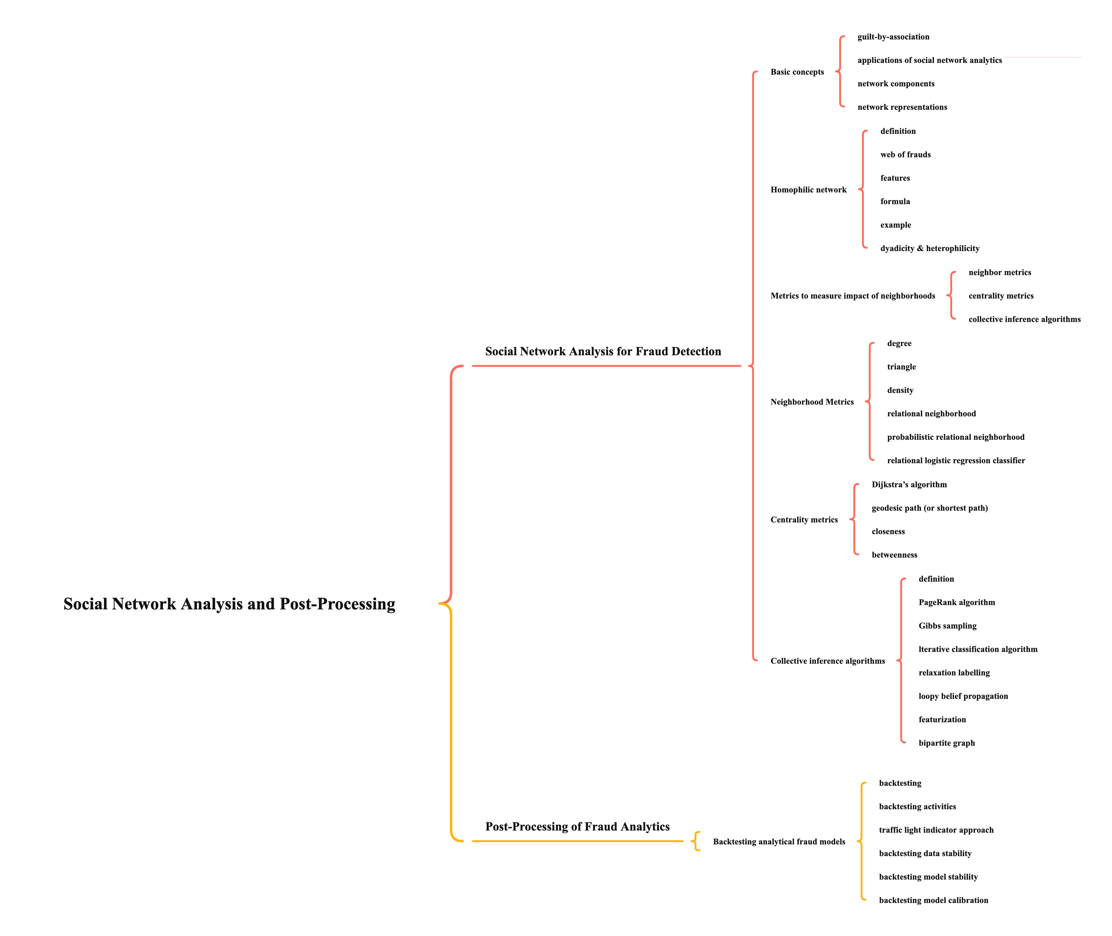
Social Network Analysis for Fraud Detection
Basic concepts
- guilt-by-association
- the reason of studying social network
- assumes that a person is guilty of a crime because he/she is associated with someone or something involved in a crime
- applications of social network analytics
- because most frauds are committed by illegal set-ups of a group of fraudsters
- traditional fraud detection models have limitations to detect relations or insight from a social network
- social network analytics will give insights about some suspicious cases (e.g., insurance frauds, bankruptcies of companies, and opinion frauds)
network components
- complex network analysis (CNA) - study of complex networks, inculding structure, characteristics, and dynamics
graph theory - mathematical study for the analysis and representation of networks
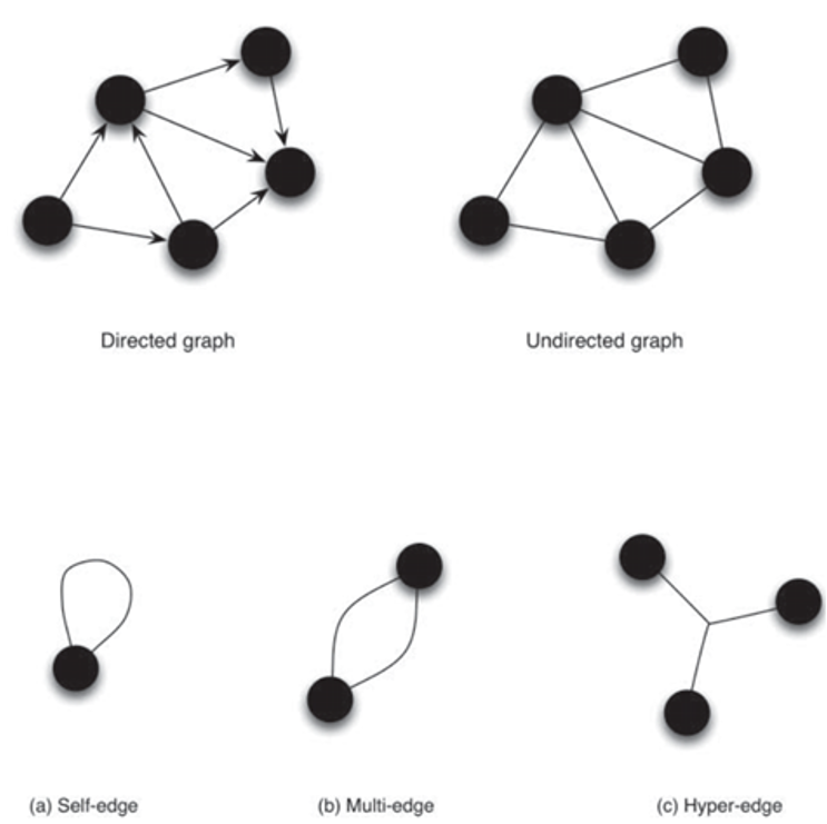
- types of graphs
- directed graph
- undirected graph
- edge representation
- self-edge - a person who transfers money from his/her account to another he/she owns
- multi-edge - a person pay the merchant money twice
- hyper-edge - 3 people attend the same event
weighted graph - represents the intensity of relations in a network
- binary weight
- 0 or 1: represents relation exists between 2 nodes or not
- -1, 0 or 1: e.g. 1 represents close relation, 0 represents no relation, -1 represents animosity
- numeric weight
- higher numeric value represents closer affinity
- normalized weight
- variant of numeric weight where all outgoing edges of a node sum up to 1
Jaccard weight
- edge weight depends on how "social" both nodes are
- formula
\[w(v_1,v_2)=\frac{|\Gamma(v_1)\cap\Gamma(v_2)|}{|\Gamma(v_1)\cup\Gamma(v_2)|}\]
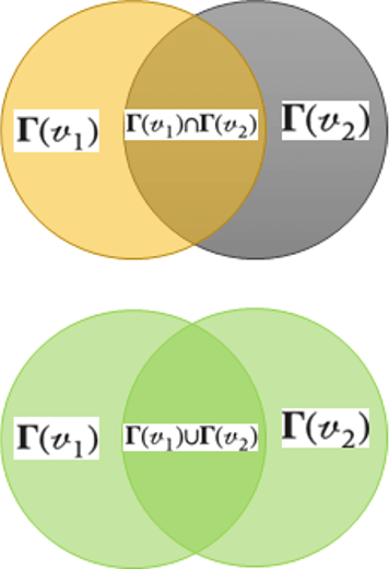
- example
- person A attended 10 events, person B attended 5 events
- both went to 3 common events
- \(Jaccard\ weight = \frac{3}{10+5-3}=\frac{1}{4}\)
- binary weight
for fraud
- nodes - legitimate or fraudulent
- edges - relationship
- egonet - one-hop neighbourhoods
- one-hop is enough for fraud analysis
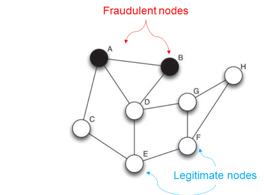
- one-hop is enough for fraud analysis
- types of graphs
network representations
- graphically (a)
- mathematically
- adjacency or connection matrix - a matrix of size \(n \times n\) (n is the number of nodes) (b)
- a sparse matrix - containing many zero values
- similar to real-life social network, where most people are only connected to a small number of friends
- adjacency list - abstract representation of adjacency matrix (d)
- weight matrix - a matrix with edge weights (c)
- weight list - abstract representation of weight matrix (e)
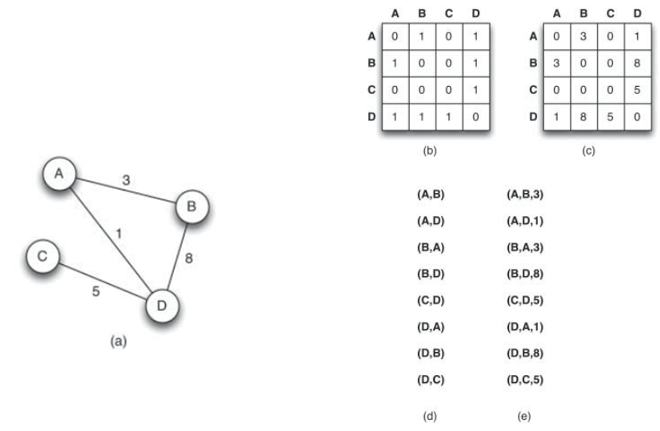
- adjacency or connection matrix - a matrix of size \(n \times n\) (n is the number of nodes) (b)
Homophilic network
- definition
- fraudsters connect to fraudsters
- legitimate people connect to legitimate people
- web of frauds
- fraudsters' nodes are grouped together
- features
- no network is perfectly homophilic - if a network exhibits evidence of homophily, it is worthwhile to investigate more thoroughly
- a network that is not homophilic is heterophilic
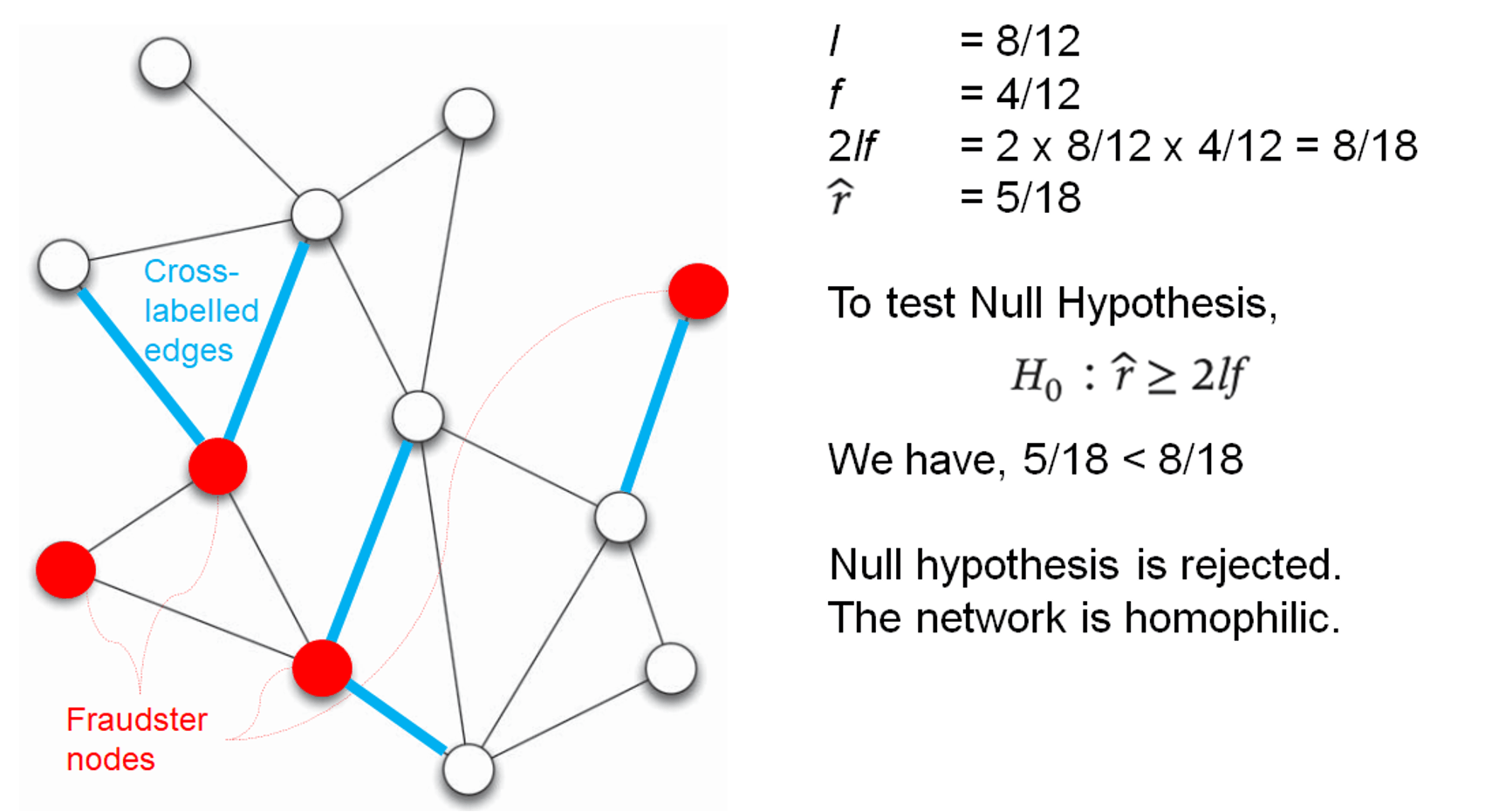
- formula
- \(l\) = legitimate nodes in the network
- \(f\) = fraudulent nodes in the network
- \(2lf\) = expected cross-label edges (fraud connects to non-fraud)
- \(\hat{r}\) = observed cross-label edges
- if null hypothesis is rejected (observed cross-label edges is significantly less than the expected cross-label edges), a network is homophilic
\[H_0 : \hat{r} \geq 2lf\]
- example
dyadicity & heterophilicity
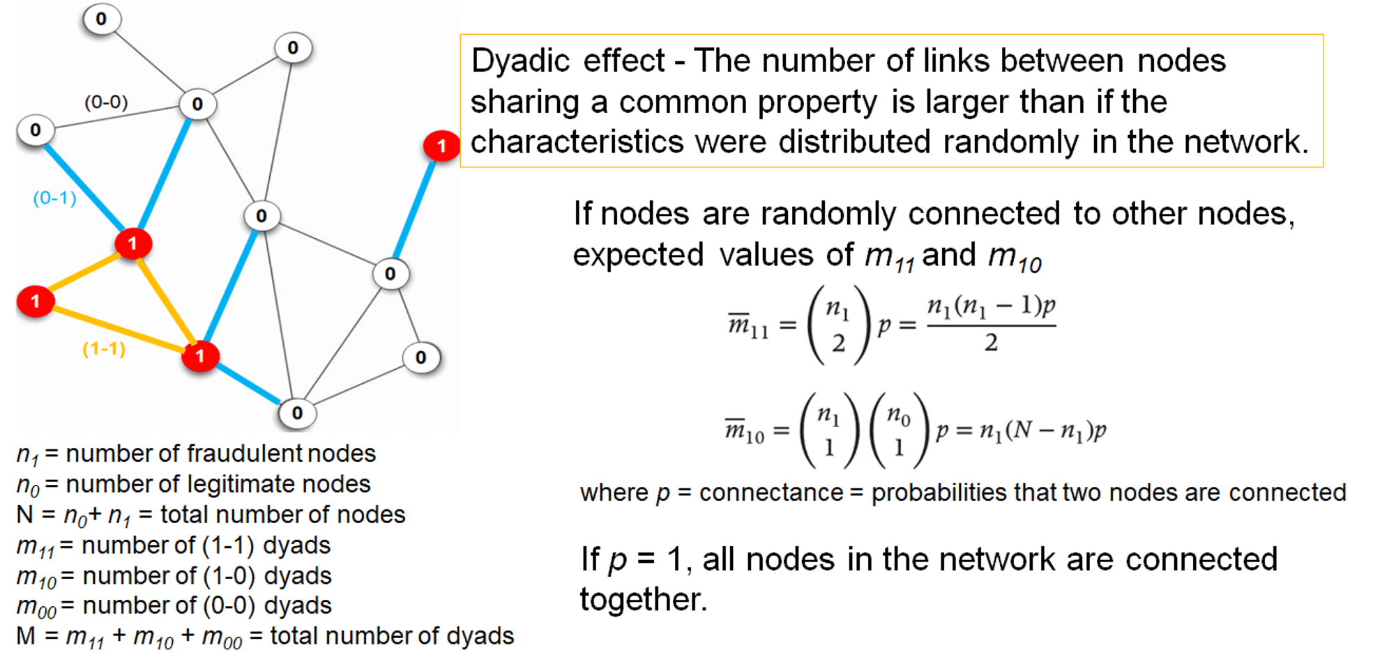
- \(Dyadicity(D)=\frac{m_{11}}{\overline{m}_{11}}\)
- \(Heterophilicity(H)=\frac{m_{10}}{\overline{m}_{10}}\)
- if D > 1, network is dyadic
- fraudulent cases tend to connect more densely among themselves than expected randomly
- if H < 1, network is heterophobic (oppsite of heterophilic)
- fraud nodes have fewer connections to legitimate nodes than expected randomly
- if a network is dyadic and heterophobic (D > 1 and H < 1), it exhibits homophily
Metrics to measure impact of neighborhoods
- neighbour metrics
- characterize the target of interest based on its direct associates
- first-order neighbour for fraud detection models
- include: degree, triangles, density, relation neighbour & probabilistic relational neighbour
- centrality metrics
- quantify the importance of an individual in a social network
- include: geodesic paths, betweenness, closeness, and graph theoretic center
- collective inference algorithms
- compute the probability that a node is exposed to fraud, i.e. probability that fraud influences a certain node
- include: PageRank, Gibbs sampling, iterative classification, relaxation labelling, and loopy belief propagation
Neighborhood Metrics
- degree
- definition
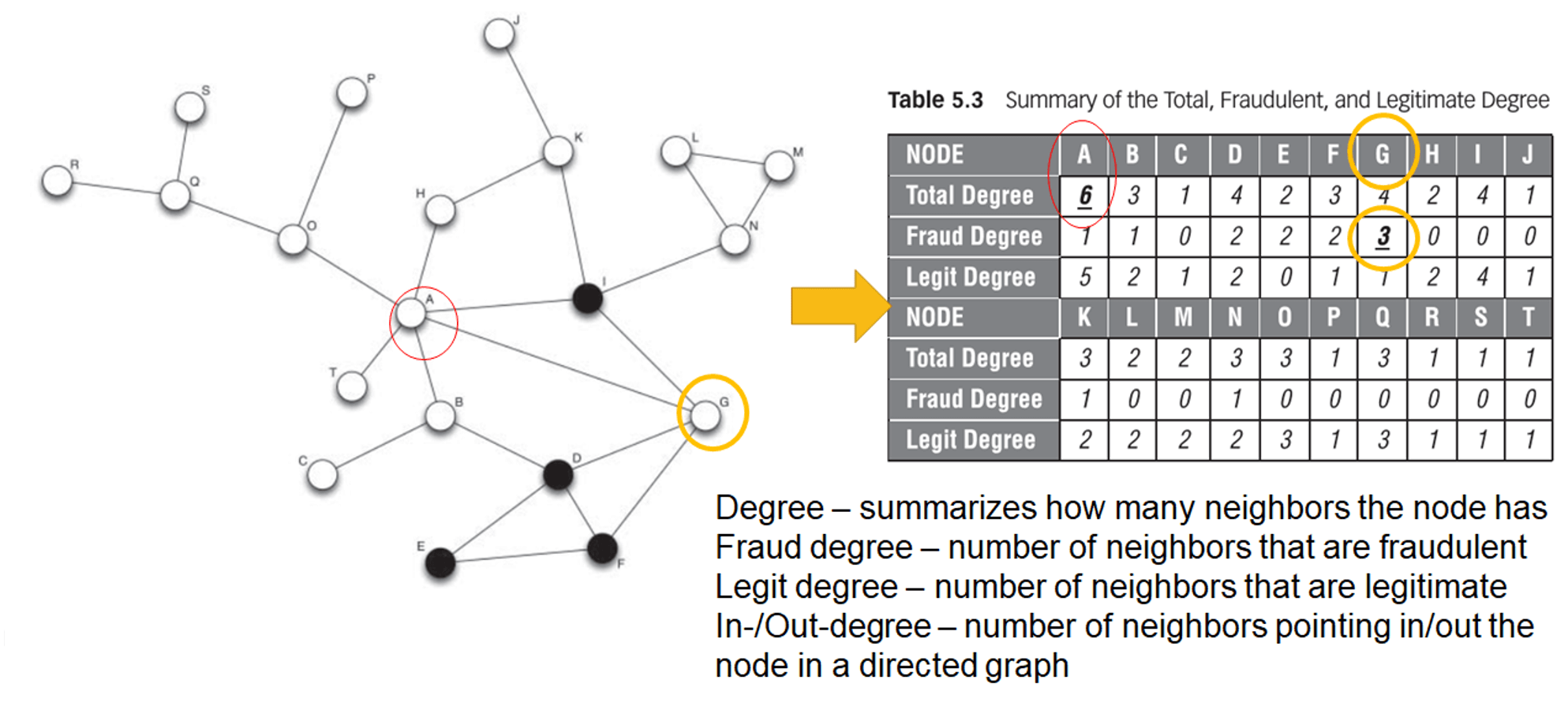
- degree distribution
- the probability distribution of the degree in the network
- in real-life networks, follows power law (i.e. many nodes are connected with few other nodes, while only few nodes are connected to many other nodes)
- k-regular graph
- network with a constant degree distribution
- each node in the network has the same degree
- e.g. 4-regular graph

- definition
- triangle
- definition
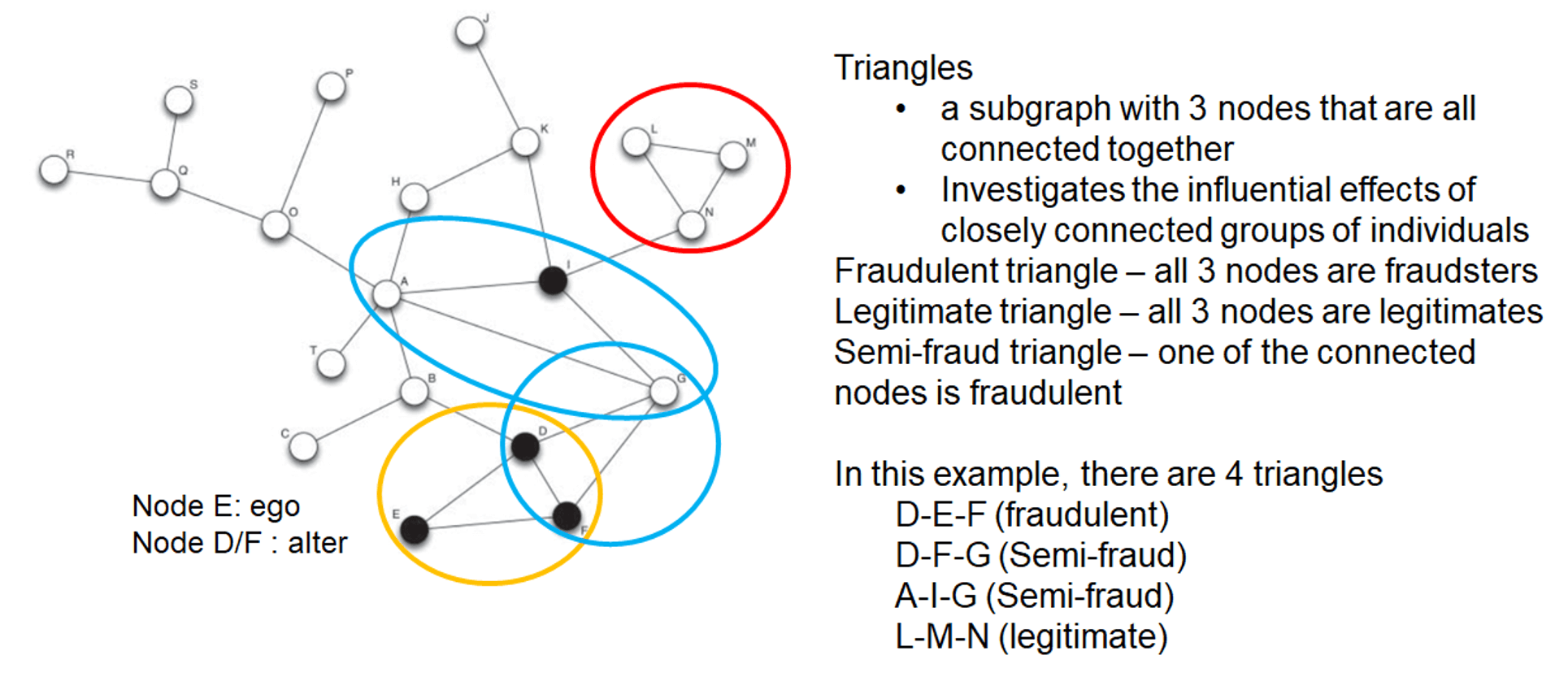
- example
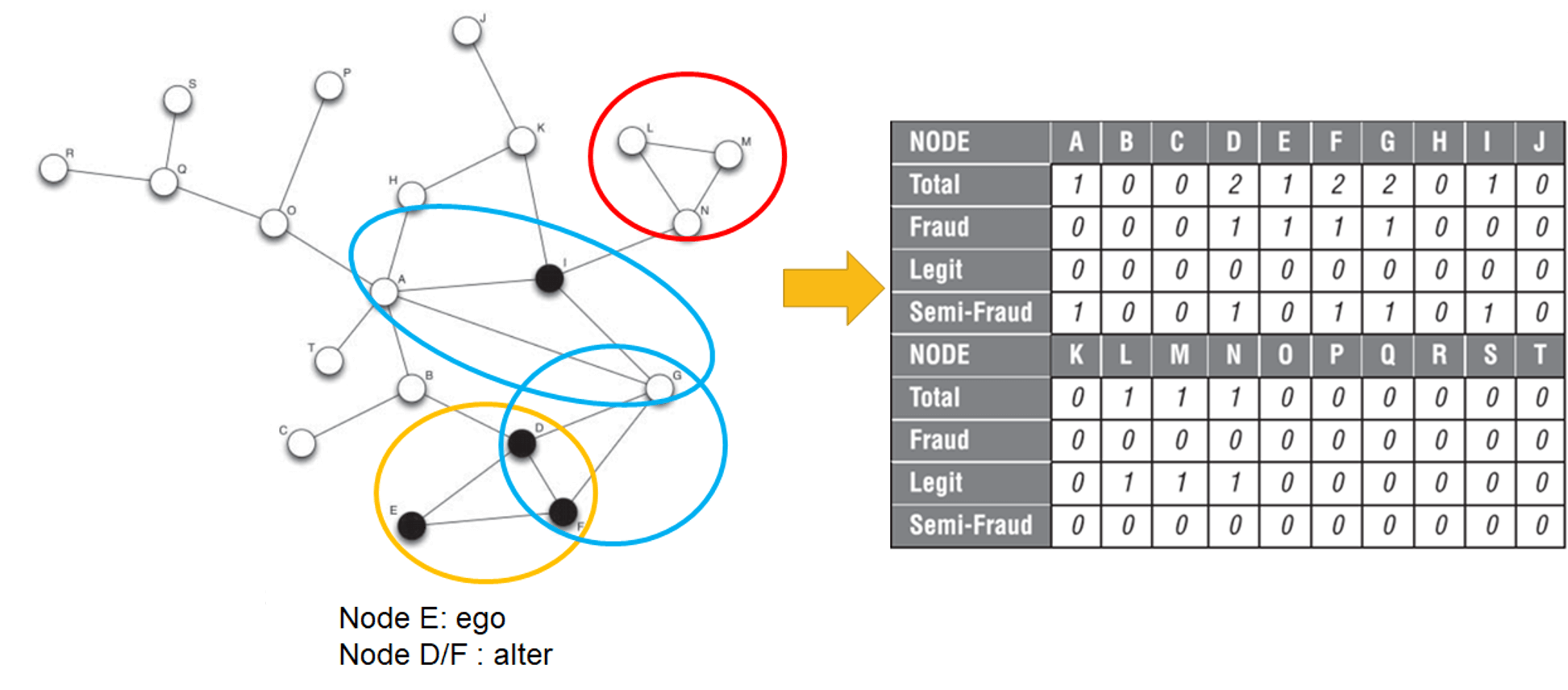
- definition
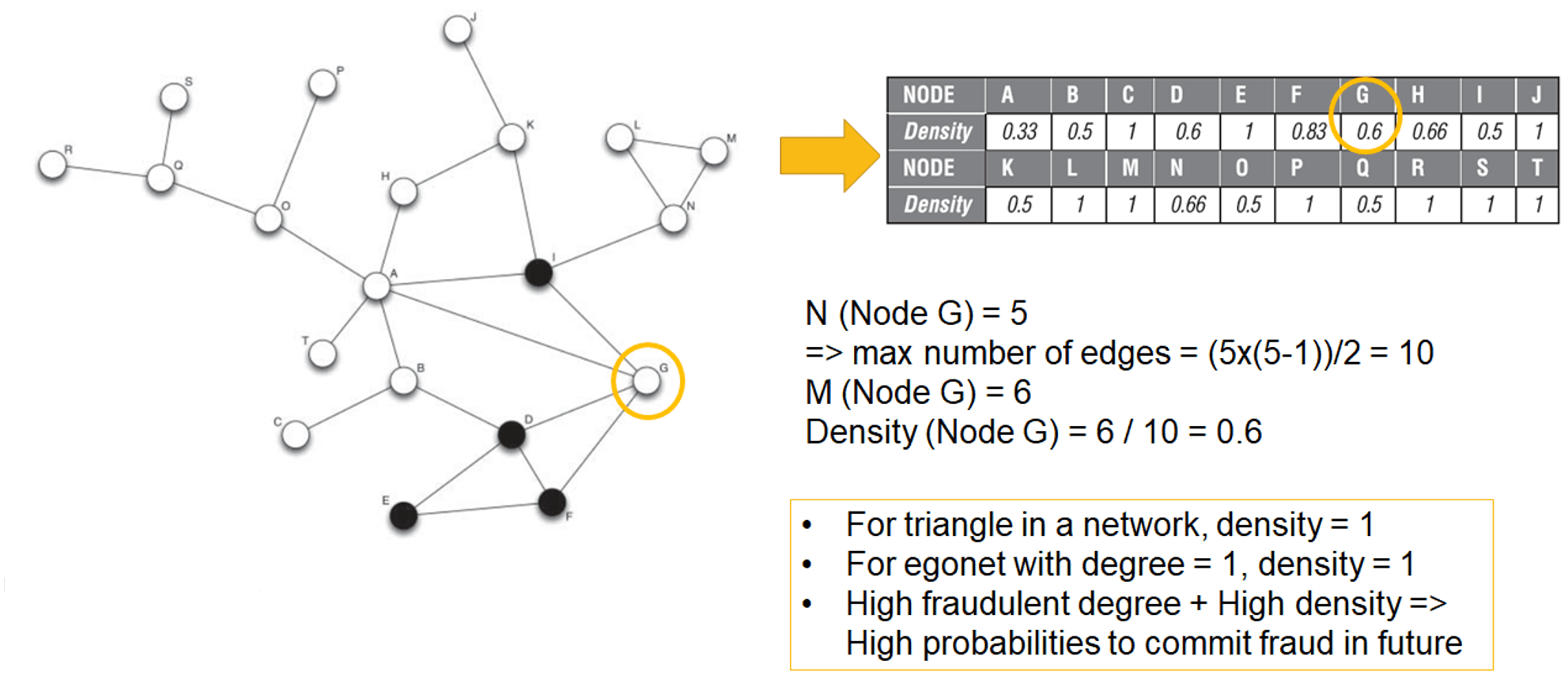
density
definition
- measures the extent to which nodes in a network are connected to each other
- i.e. measures the number of observed edges (M) to the maximum possible number of edges in the graph
- full connected network: each node is connected to every other node, has \(\frac{N(N-1)}{2}\) edges, where N = total number of nodes
\[d=\frac{2M}{N(N-1)}\]
example
relational neighbourhood
- relational neighbor classifier
- makes use of the homophily assumption - connected nodes have a propensity to belong to the same class, i.e. guilt-by-association
- if two nodes are associated, they tend to exhibit similar behaviours
- posterior class probability for node n to belong to class c
- example
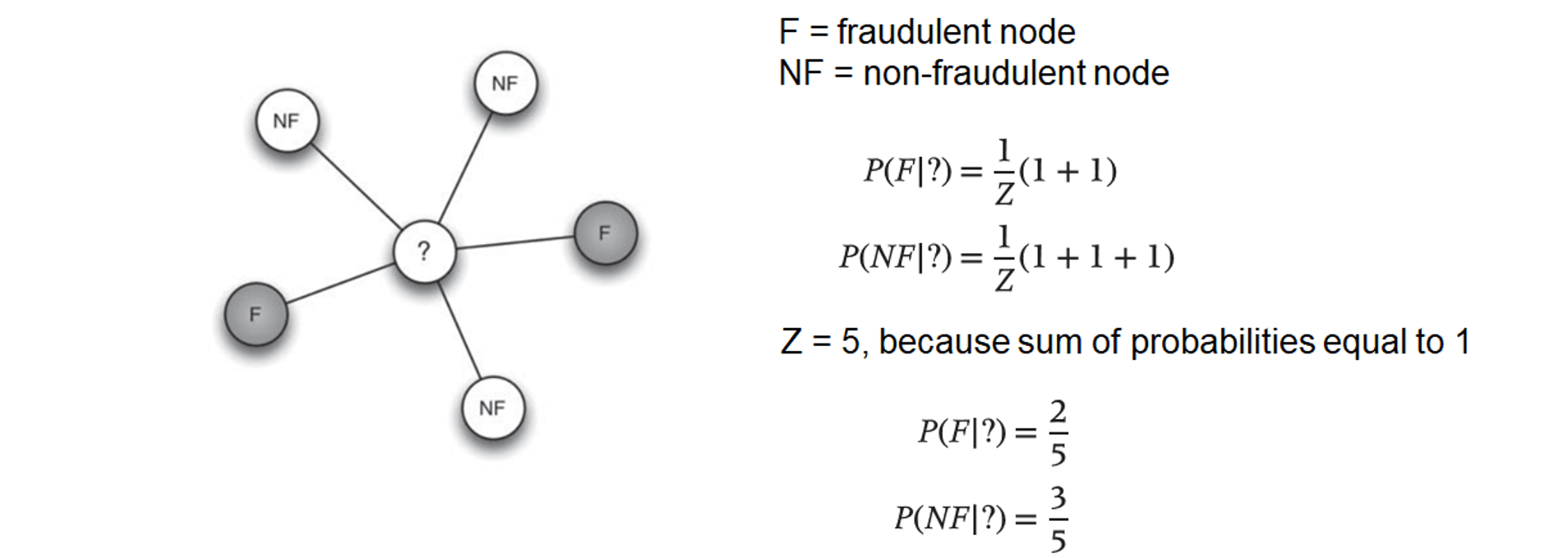
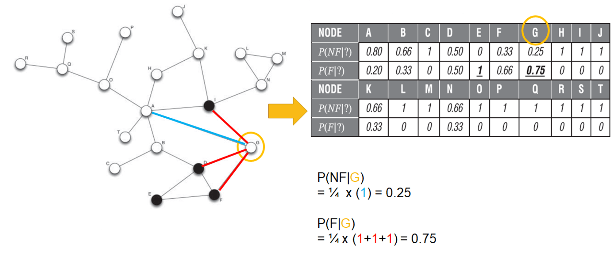
- example
- relational neighbor classifier
probabilistic relational neighborhood
- extension of relational neighbour classifier
- example
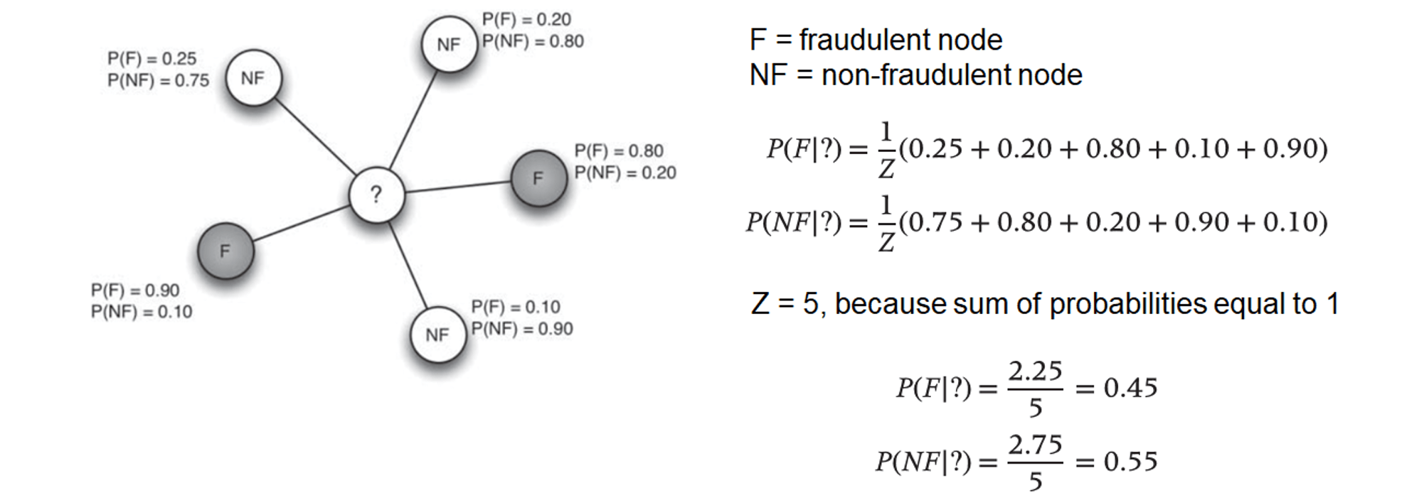
- \(P(c|n_j)\) can be result of a local model, or of a previously applied network model
- relational neighborhood and probabilistic relational neighborhood, can both be used as a classifier, or an additional variable in fraud prediction models
relational logistic regression classifier
- definition
- starts with a dataset with local node-specific characteristics called, intrinsic variables, e.g. company's age, sector, etc.
- network characteristics
- mode-link: most frequently occuring class of neighbor
- count-link: frequency of the classes of the neighbor
- binary-link: binary indicators indicating class presence
- example

- trick: use logistic regression with the dataset that contains both intrinsic and network variables
- caution: there might be correlations between the network variables added
- filtered out during an input selection procedure (e.g. using stepwise logistic regression), or
- featurization - can measure the behaviour of the neighbors in terms of the target variables or the intrinsic variables
- definition
Centrality metrics
- Dijkstra's algorithm
- example
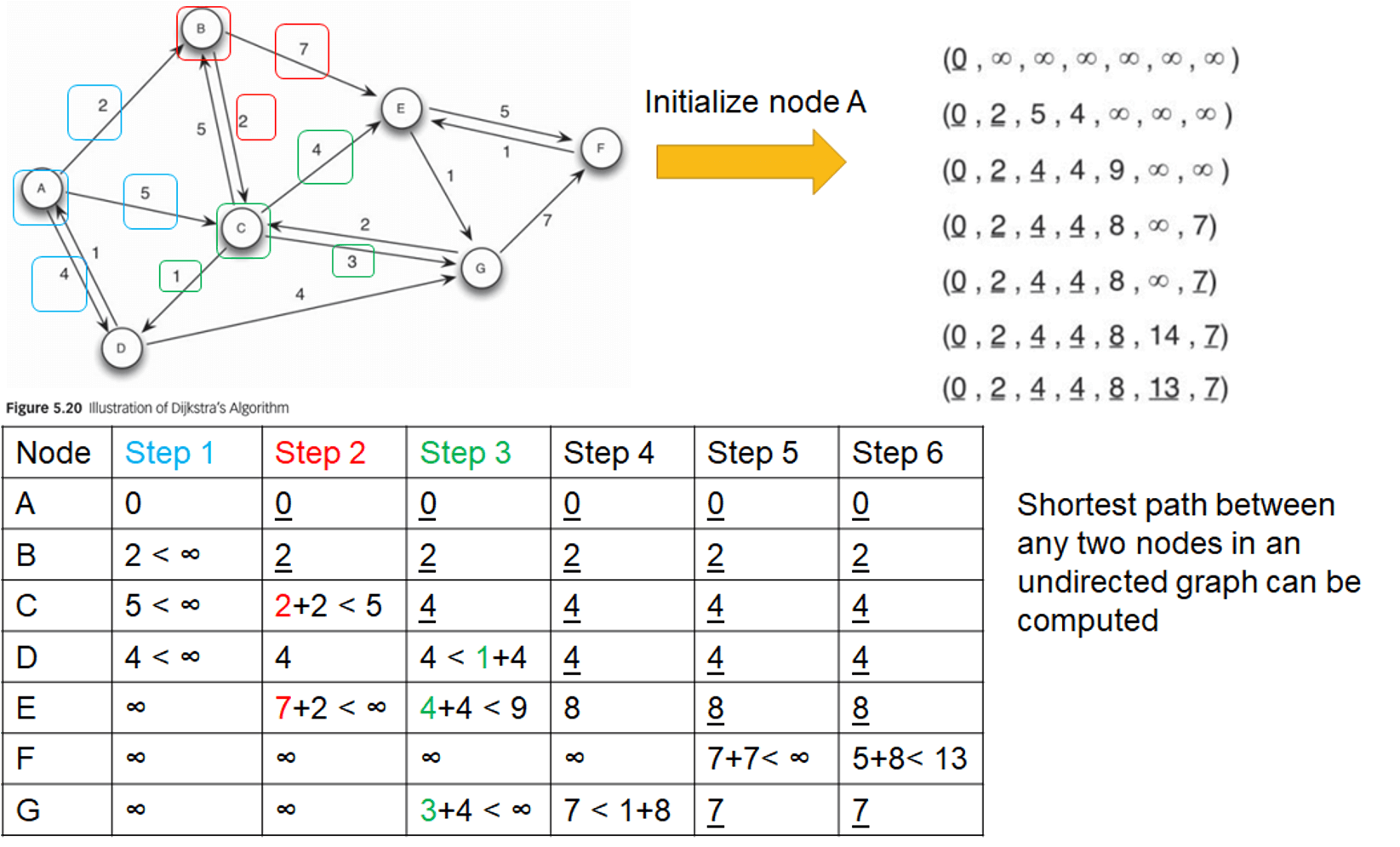
- Dijkstra's algorithm is only applicable to networks with non-negative edge weights
- example
- geodesic path (or shortest path)
- computes the minimum distance needed to reach a node from a target node
- Q: how far is any fraudulent node in the network removed from the target node?
- if a fraudulent node is in the close neighborhood, fraud might impact the node more intensively and contaminate the target of interest
- graph theoretic center
- the node with the smallest, maximum distance to all other nodes, i.e. most central node in the network
- average path length
- length one needs to traverse on average to reach one node from another
- in fraud, if more paths exist between two nodes, there is a higher chance that fraudulent influence will eventually reach the target node
- adjacency matrix - number of connecting paths between any two nodes
- example
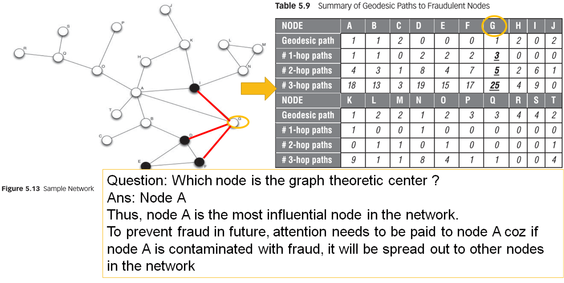
- example
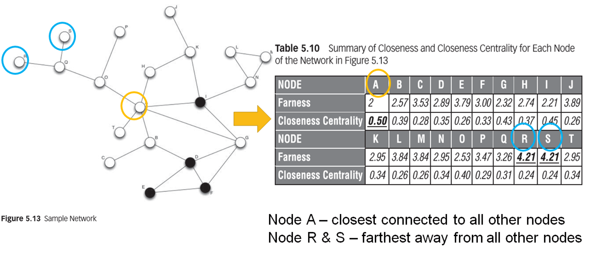
closeness
definition
- mean geodesic distance or farness measure
- \(d(v_i v_j)\) = distance between a node and another node corresponds to the geodesic or shortest path
- \(g(v_i)\) = mean geodesic distance or farness from a node i to the other nodes
- \(n\) = number of nodes in a network
\[g(v_i)=\frac{\displaystyle \sum_{j=1(j\neq i)}d(v_i v_j)}{n-1}\]
- mean geodesic distance or farness measure
closeness centrality
- measures the mean distance from a node to each other in the network
- inverse of farness measure
\[Closeness \ Centrality(v_i)={(\frac{\displaystyle \sum_{j=1(j\neq i)}d(v_i v_j)}{n-1})}^{-1}\]
a few points to note
- the higher the value, the more central the node is in the network
- the value of closeness centralities for all nodes in the network might lie closely together, and therefore important to inspect the decimals
- closeness centralities often excludes the distances to nodes that cannot be reached
example
betweenness
- definition
- measures the extent to which a node lies on the geodesic paths connecting any two nodes in the network
- the extent to which information passes through this node
- a node with a high betweenness possibly connects communities with each other
betweenness centrality
- \(g_{jk}\) = number of shortest paths between node j and node k
- \(g_{jk}(v_i)\) = number of shortest paths between node j and node k that pass through node \(v_i\)
\[\displaystyle \sum_{j < k}\frac{g_{jk}(v_i)}{g_{jk}}\]
example
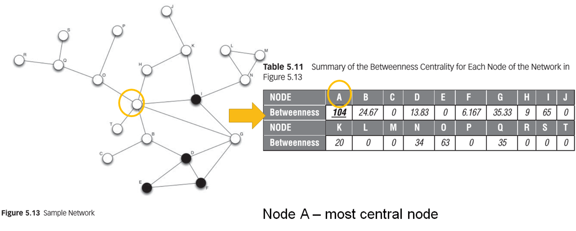
- definition
Collective inference algorithms
- definition
- infers a set of class labels/probabilities for the unknown nodes
- rationale: inferences about nodes can mutually affect one another
- PageRank algorithm
- Google based on this
- explaination
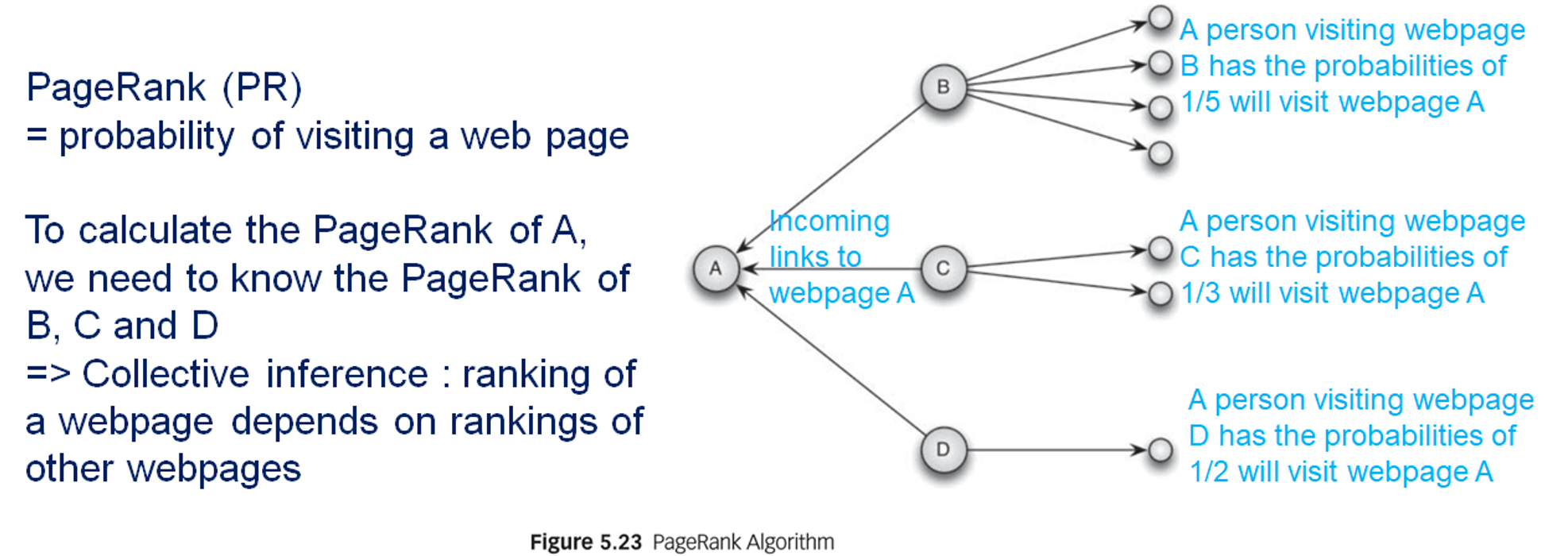
- ranking of a web page depends on
- ranking of web pages pointing towards that web page
- out-degree of the linking web pages
- random surfer: assumes surfers get bored and jumped randomly to another web page
- to calculate the PageRank requires ranking of the neighboring web pages
- start with a random RageRank value for every web page
- lteratively update the PageRank scores until a predefined number of iterations is reached, or a stopping criteria is met (e.g. when the change in the ranking is marginal)
- application of PageRank algorithm to fraud analytics
- PageRank algorithm can be seen as a propagation of page influence through the network
- propagate fraud through the network
- personalize PageRank by fraud
- i.e. adjacency matrix A = fraud network (i.e. people-to-people network)
- example
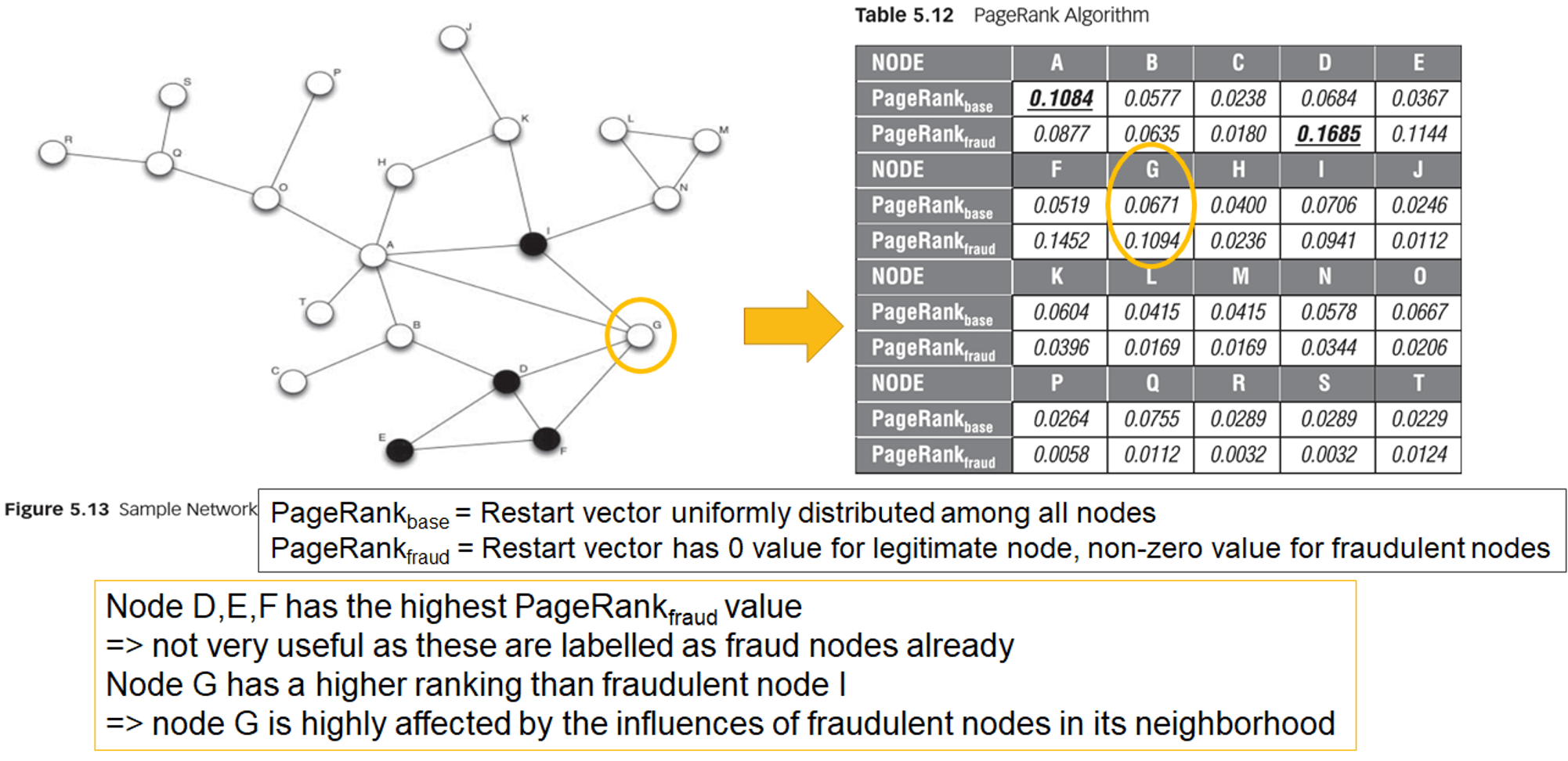
- Gibbs sampling
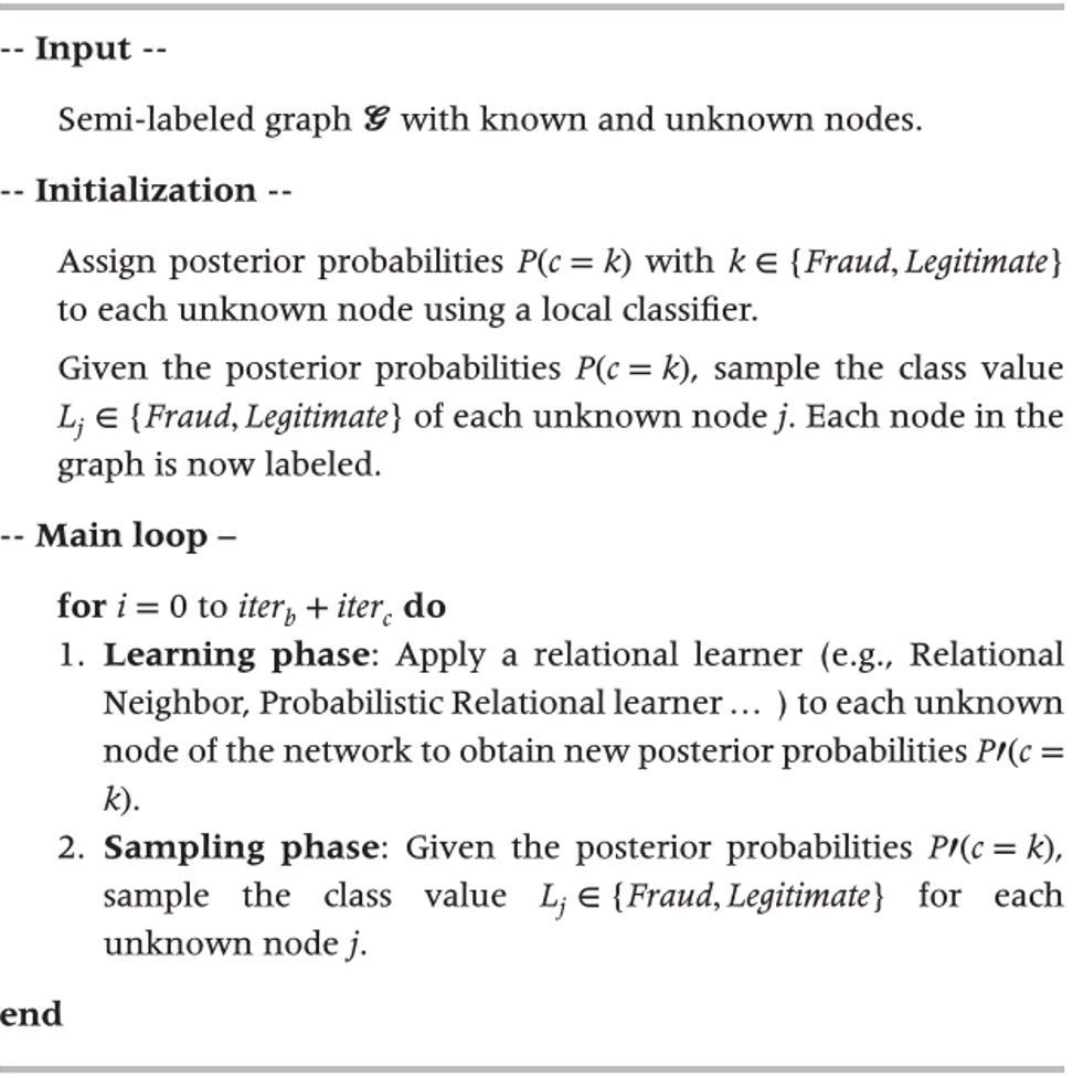
- uses a local classifier to infer a posterior class probability in order to initialize the node labels in the network
- original semi-labelled graph is transformed in a fully labelled graph by sampling the posterior probabilities of the local classifier
- predictive features of a local classifier consist of only intrinsic variables
- labels of unknown nodes in the graph express an expectation of the true class value
- lterative procedure
- updates the expected class labels of the unknown nodes
- the first \(iter_b\) steps approach a stationary distribution (burn-in period), where no statistics are recorded
- the last \(iter_c\) steps, keeps track of which class labels are assigned to each node
- final class probability estimate is computed as normalized count of the number of times each class is assigned to a particular node
- lterative classification algorithm
- similar to Gibbs sampling, iterative classification initializes the semi-labelled graph by using a local classifier
- bootstrap phase
- based on the local model’s output, the most probable class label is assigned to each unknown node
- iteration phase
- a relational learner updates the class labels of each unknown node based on the outcome of a relational logistic regression model
- input features: computed as link statistics of the current label assignments
- link statistics: mode (most occurring label of the neighboring nodes), count (number of neighboring fraud nodes), binary (at least one of the neighboring nodes are fraudulent)
- nodes not yet classified are ignored
- a new class label is assigned to each unknown node based on the largest posterior probability, this step is repeated until a stopping criterion is met
- the final class label corresponds to the class label estimate generated during the last iteration
- relaxation labelling
- starts from a local classifier to initialize a node’s class label
- previous approaches assigned a hard label (i.e. either legitimate or fraud).
- soft labelling: relaxation labelling starts with assigning each node a probability that indicates the likelihood of a node to belong to a certain class
- next, the probability class labels are used to iteratively update the class probability using a relational model
- the class estimates of the last iteration are the final class label estimates
- loopy belief propagation
- a collective inference procedure based on iterative message passing
- idea
- belief of each node to be in state x (let’s say fraud) depends on the messages it receives from its neighbors
- belief of a node to be in state x is the normalized product of the received messages
- the message as well as the belief is continuously updated during the algorithm
- featurization
- mapping of an unstructured data source like a network into useful and meaningful characteristics of each node
- most network-based features already give a good indication which nodes might be fraudulent in the future, these network-based characteristics can be combined with local features into a classification model
- bipartite graph
- unipartite network
- networks with only one node type
- link weight: shared events or behaviors
- the higher the link weight, the more intense the relationship is
- two nodes are more influenced by each other if their relationship is more intense
- affiliation or bipartite network
- represent the reason why people connect to each other, and include the events that network nodes (e.g. people or company) attend or share
- creates new insights in the network structure

- unipartite network
Post-Processing of Fraud Analytics
Backtesting analytical fraud models
- backtesting
- aims at contrasting ex-ante made predictions with ex-post realized outcomes
- key idea is to verify whether the fraud model still performs satisfactory
- important because fraudsters might outsmart fraud analytical models by continuously changing their strategies

- backtesting activities
- data stability
- model stability
- model calibration
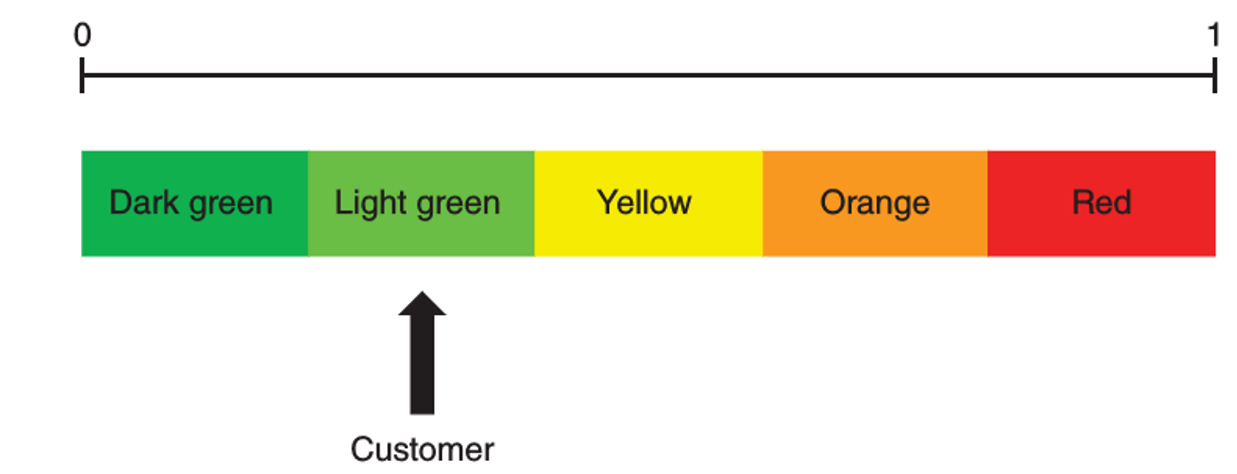
- traffic light indicator approach
- green light = low probability of fraud
- red light = high probability of fraud
backtesting data stability
- check whether the population on which the model is currently being used is similar to the population what was used to develop the model
- if difference occur in step 1, verify the stability of the individual variables
for step 1, a system stability index (SSI) can be calculated as
\[SSI=\sum_{i=1}^k(observed_i - expected_i).ln\frac{observed_i}{expected_i}\]
- SSI measures difference between expected and observed distribution
- higher SSI implies a population shift and instability
- rule of thumb
- SSI < 0.10: no significant shift (green)
- 0.10 ≤ SSI < 0.25: moderate shift (yellow)
- SSI ≥ 0.25: significant shift (red)
- SSI also referred to as deviation index, identical to information value
- SSI can be monitored through time or by individual variables
backtesting model stability
- volatility of the model performance
- to track the model performance using PM (performance metric), no. of observations, no. of frauds and corresponding traffic light
- to track over a subsequent peroid of time
- traffic light coding procedure
- if change of PM < 5%, assign green light
- if change of PM ≥ 5% and < 10%, assign yellow light
- if change of PM ≥ 10%, assign red light
- bootstrapping procedure
- pool the training and out-of-time test observations with the predicted PM into one larger sample
- draw a training and a test set bootstrap sample with the same size as the original training and out-of-time test set (NOTE: a bootstrap sample is one with replacement)
- calculate the difference for PM between the bootstrap training and the bootstrap test sample
- repeat 1,000 or more times to get the distribution and statistically test whether the difference is zero
- traffic light procedure
- green: no statistical difference at 95%
- yellow: statistical difference at 95% but not at 99%
- red: statistical difference at 99%
backtesting model calibration
- in classification or regression model
- aim of the model is to come up with well-calibrated estimates of fraud probabilities or fraud amounts
- the calibration needs to be monitored in time
- procedure
- a classification model assigns fraud probabilities to various pools of customers
- each pool has a corresponding calibrated probability, as it was calculated during model development
- to see how these probabilities evolve in time and whether they remain stable
- binomial test
- used as heuristic for evaluating the quality of the calibration
- traffic light procedure
- green: no statistical difference at 90%
- yellow: statistical difference at 90% but not at 95%
- orange: statistical difference at 95% but not at 99%
- red: statistical difference at 99%
- hosmer-lemeshow test
- test calibrated versus observed fraud rates across multiple pools simultaneously
- backtest calibration of regression model
- use a parametric student's t-test
- can be used to evaluate the significance of the error defined as the difference between the amount predicted and observed
- output of regression model has been categorized into pools
- use a parametric student's t-test
- in classification or regression model
fite7410 financial fraud analytics fintech social network post-processing
2484 Words
2021-03-20 16:08